Week 5 - Rayleigh Taylor Instability

Rayleigh Taylor Instabilities

Aim: The main aim of this project is to observe the Rayleigh instabilities between two fluids, lying one above the other with fluid with the higher density above. The comparison was made by changing the grid size and changing the heavier fluid with respect to time.

Introduction: The formation of instabilities when the fluids with two different densities interact with each other can be visualized by Raleigh-Taylor instabilities, these instabilities are the result of buoyancy forces and surface tension forces between them. The surface tension is the tensile force between the two fluid layers is a result of cohesion and the adhesion between the fluid molecules. Whereas the buoyancy forces arise when there is a density difference and between two fluids and the lighter fluid tends to rise against the attraction of gravitational pull. The buoyancy force tends to destabilize the fluids whereas the surface tension causes the fluid to stabilize. The overall result of what happens when two fluids of different densities interact with each other can be predicted by a non dimensional number called “Atwood- number”

Which is given by the relation

Where rho_1 is density of the upper fluid ,

and rho_2 is density of the lower fluid.

If the Atwood number is negative, the system is destabilizing else its stabilizing.

Methodology

For this assignment, we start with generating a 2D model in space claim in the following steps

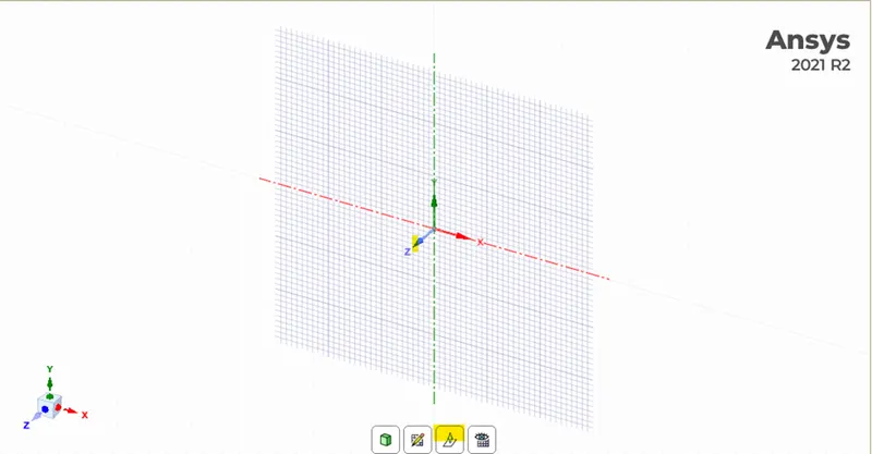
Step 1 open the space claim and select the XY 2D plane as shown

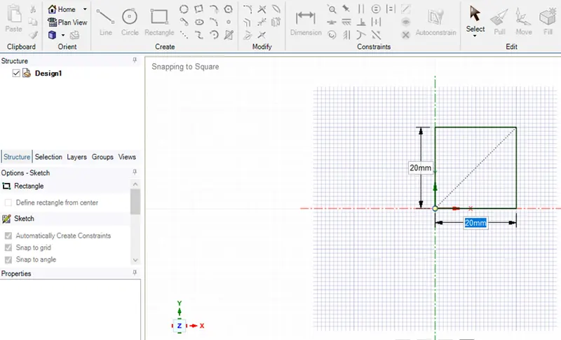
Step 2 By clicking the rectangle icon generate a 20 mm by 20mm square as shown above.

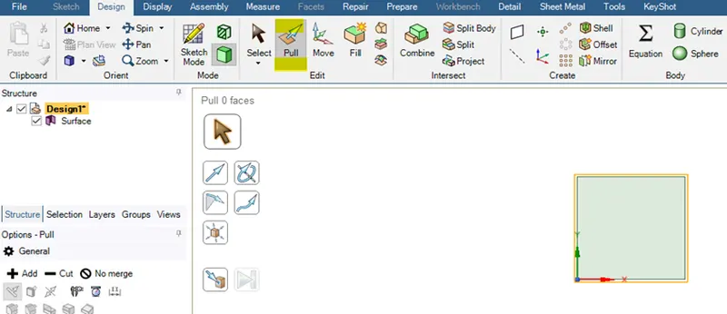
Step 3. Using the workbench from toolbar select the pull option , which generates a surface .

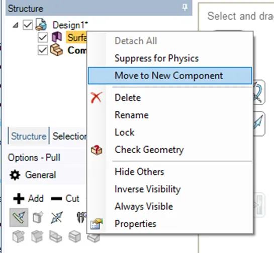
Step 4. Using the move to new component and name that as air

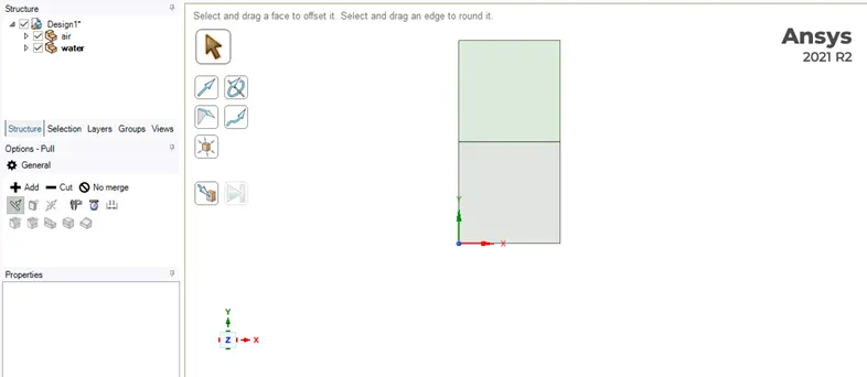
Step 5. Using the steps 2 -4 generate a new surface above the air name it as water

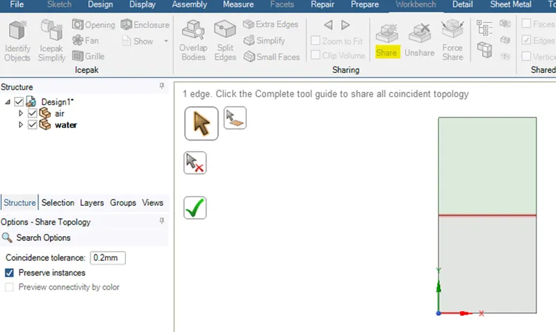
Step 6. Using the Workbench from the toolbar, click the share topology.

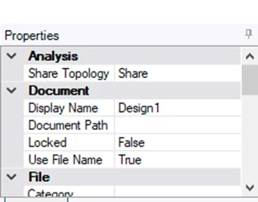
Step 7.By clicking the properties, we can see under Share Topology it shows Share

Meshing

Closing the space claim window and starting meshing, using the double precision and parallel by selecting the number of processors.

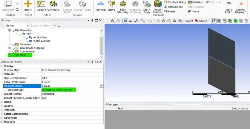
Step 1 By clicking the mesh and generating the mesh initially with a size of 0.5 mm .

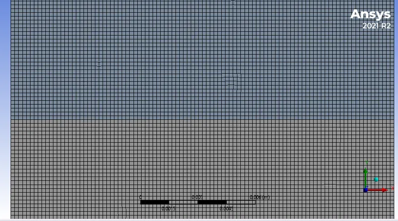
Mesh if it is changed to 0.2 mm

Fluent

Closing the meshing window and opening the fluent by using the setup from the workbench window.

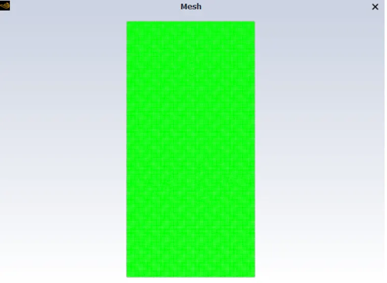
The uploaded mesh in the fluent is displayed as above

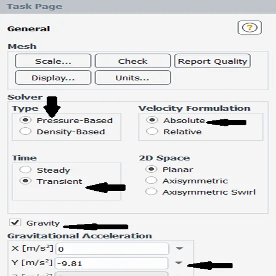
Step 1: From the Task Page select the solver as Pressure Based and Velocity formulation as Absolute and a Transient Solver , 2D Space Planar , Selecting the Gravity and gravitational acceleration as -9.81 m/s2

Step 2: From the Physics tab in the toolbar select Multiphase

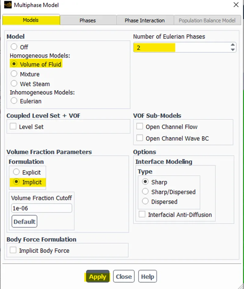
Step 3: From the models select Volume of Fluid, number of Eulerian Phases as 2, since we are using 2 types of fluids water and air. Selecting the volume fraction parameters as Implicit which is unconditionally stable model.

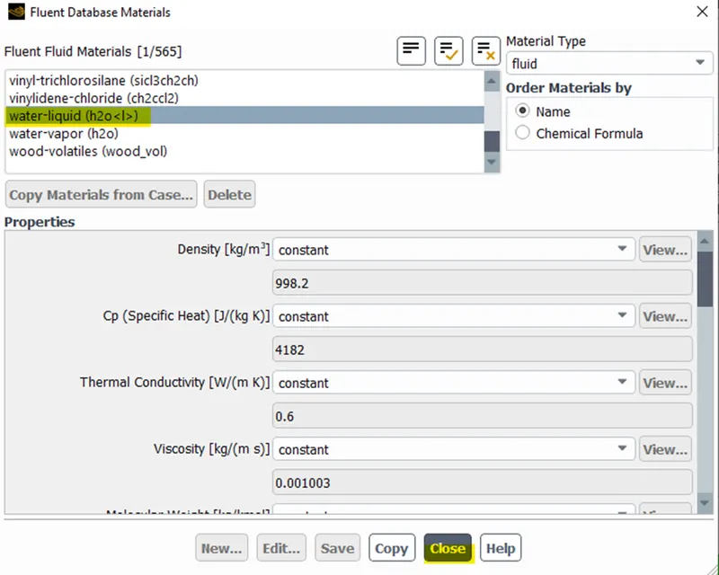
Step 4: from the materials tab in the toolbar, selecting Fluent Database and selecting the water-liquid and clicking copy and close.

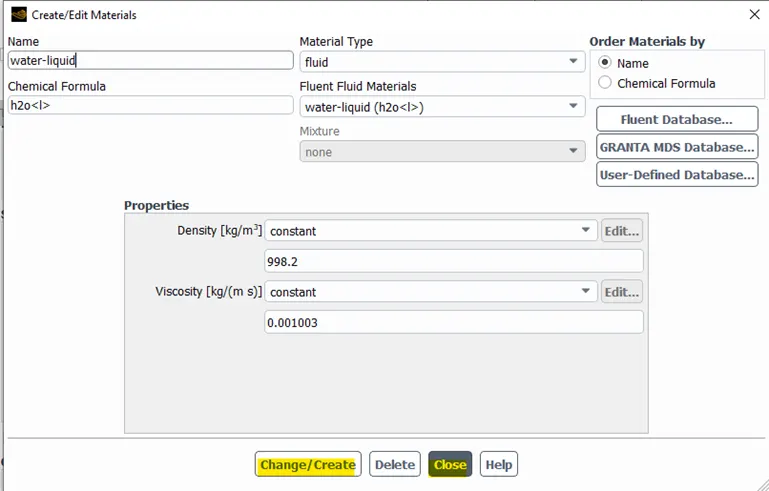
That will be appeared in the materials .

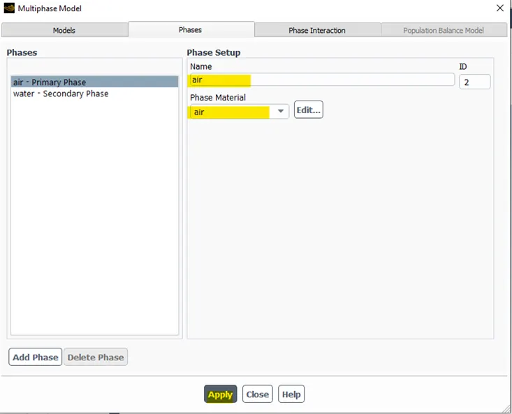
Step 4: From the Multiphase Model select the phases as air as Primary Phase and water as Secondary Phase.

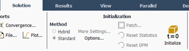
Step 5: Initializing the solution by clicking Initialize

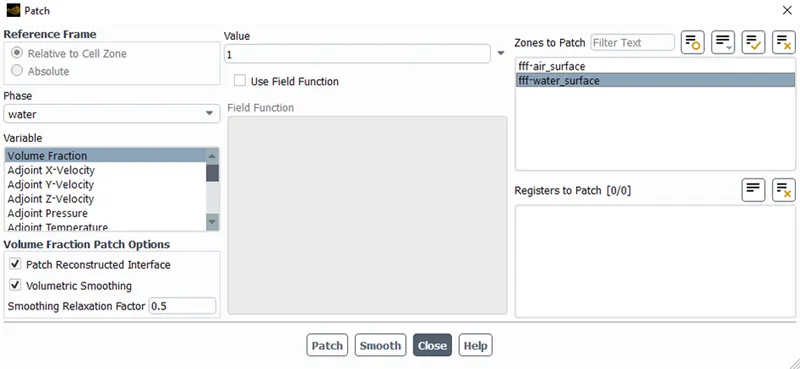
Step 6: Clicking the patch for selecting the surfaces of air and water in mesh and with volume fraction as 0 and 1 as follows and clicking patch after each operation

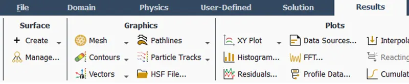
Step 7: Now clicking the contours, we create a volume fraction contours for the surfaces water and air

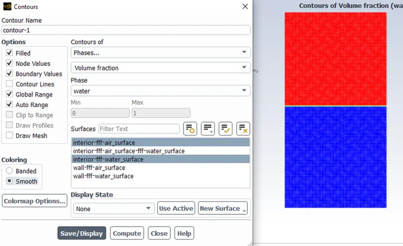
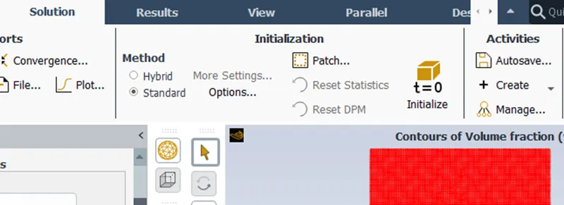
Step 8: For creating animation of volume fraction we need click Create from Activities and selecting the contour of volume fraction.

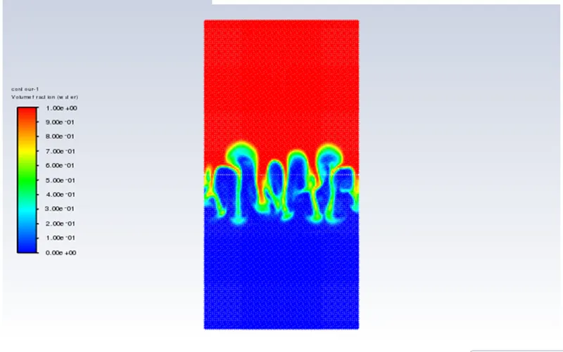
The animation and residuals

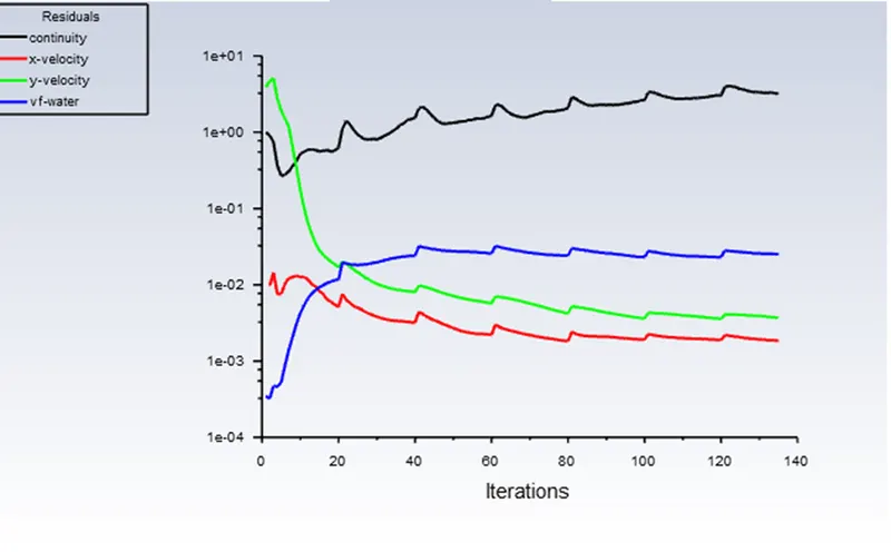
The solution converged at around 140 iterations

For Finer Grid

For finer grid we go to the meshing part and change the element size to 0.2 mm instead, and the same simulation is repeated , but following errors were incurred during that solution.

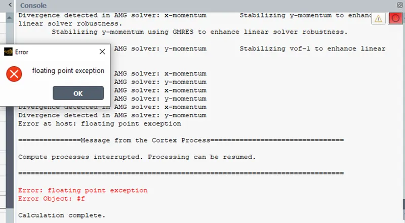
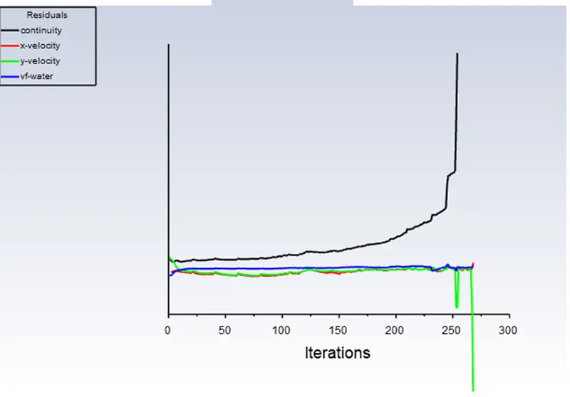
Residuals are unstable

Under solution Tab , Click controls and

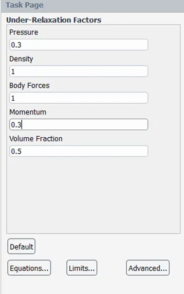
Change the value of pressure and momentum to 0.3, and run the solution again

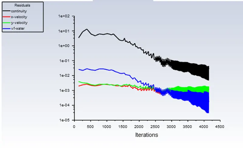
Solution was converged at 4300 iterations, with a time step size of 0.02

Using User defined Material instead of water

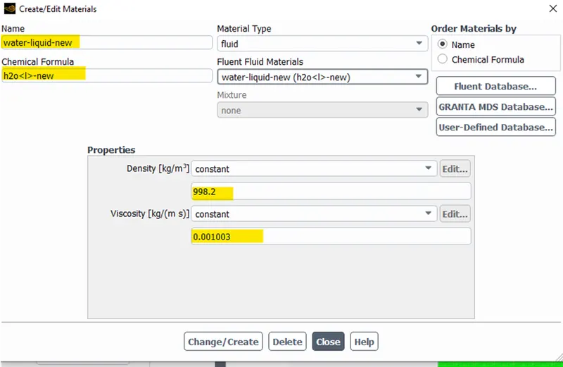
The values and names highlighted are changed accordingly as below

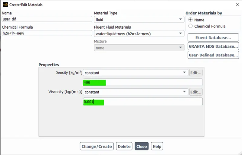
And solved till the convergence reached by repeating steps in the fluent.

Comparison of the Rayleigh Instability

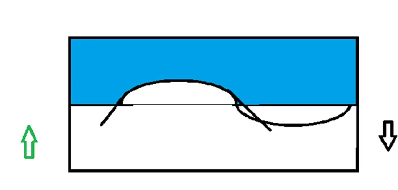
The above figure shows the perturbations that occur during the instabilities initially, the gravitation force acts downwards whereas the buoyancy forces act upward direction and finally the surface tension forces acting tangentially on the layer such that pulling back to its initial state, the surface tension causes a stabilizing effect whereas the buoyancy causes the destabilizing effect.

The perturbations are in the form of waves with wavelength “λ”, from this we solve the surface tension effects on fluid layers, which is given by

Surface Tension ≈ γ.a .k²

Where a is the amplitude of the perturbations.

And k is the reciprocal of the wavelength.

The conservation laws

`∂(ρY_i)/(∂t)+∇⋅(ρY_i.u+J_i)=0 ; (i=1,2)`

`∂(ρu)/( ∂t)+∇⋅[ρu⃗ u⃗ +pδ⃗ →−τ⃗ →]=ρg⃗`

`∂E/(∂t)+∇⋅[(E+p)u⃗ −τ⃗ →⋅u⃗ +q⃗ c+q⃗ d]=ρg⃗ ⋅u⃗`

where ρ is density, Yi is the mass fraction of species i , u is velocity, J i=−ρD∇Yi is a diffusional mass flux (where D is binary diffusivity), p is pressure, δ is the unit tensor, τ → is the viscous stress tensor g is gravity (or frame acceleration), E=ρ(e+u⃗ ⋅u⃗ /2) is total energy (with e being internal energy), q⃗ c is the conductive heat flux and q⃗ d is enthalpy diffusion (Bird et al. 1960). Closure of the above equations requires an equation of state for both fluids.

• it is observed the instabilities are shown for a larger time in comparison with coarse grid size.
• its also seen that the instabilities are diffused since the presence of fewer elements.
• Buoyancy forces causing the instabilities in the domain.
• Surface tension forces caused the stabilizing the domain.
• It take much time for the convergence in the casea of finer grid.
• It takes lesser time for convergence in the coarse grid.
• Domain reaches the stable condition, quicky in coarse whereas slowly in a finer grid.
• The atwood number is 0.997, since water is fluid in both cases.

• Since the lower density of the user-defined fluid the buoyancy forces are lesser in comparison with water.
• its also seen that the time taken for settling the perturbation is lesser in case of water than user defined fluid.
• Buoyancy forces causing the instabilities in the domain.
• Surface tension forces caused the stabilizing the domain.
• The convergence time is more or less the same in both cases.
• Both cases are unstable when using with finer grid size and modifications were made to make solution stable.
• The atwood number is 0.997 for water and 0.995 for user defined fluid. That is our atwood number for user defined fluid is slightly lesser than water