Week 3.5 - Deriving 4th order approximation of a 2nd order derivative using Taylor Table method

For calculating the second order derivative of the given function at fourth order approximation , we need to solve a set of finite difference eqautions,

But firstly we need to find the number of nodes in the stencil for each kind of scheme

1. Central Difference
2. Skewed right
3. Skewed Left

CENTRAL DIFFERENCE SCHEME

for scheme 1 the number of nodes on the stencil is given by

N = P+Q -1

P = order of approximation in our case its 4

Q = order of derivative we require 2nd order derivative

N = 4+2-1 = 5 are the no of nodes on stencil

so we need to use the difference equations for 2 nodes away from each side of the point

`f(i-2) = f- (delf)/(delx)(2deltax)+(del^2f)/(delx^2)(((2deltax)^2)/(2!))-(del^3f)/(delx^3)(((2deltax)^3)/(3!))+(del^4f)/(delx^4)(((2deltax)^4)/(4!))``

`f(i-1) = f- (delf)/(delx)(deltax)+(del^2f)/(delx^2)((deltax^2)/(2!))-(del^3f)/(delx^3)((deltax^3)/(3!))+(del^4f)/(delx^4)((deltax^4)/(4!))-(del^5f)/(delx^5)((deltax^5)/(5!))``

`f(i)=f`

f(i+1) = `f+ (delf)/(delx)(deltax)+(del^2f)/(delx^2)((deltax^2)/(2!))+(del^3f)/(delx^3)((deltax^3)/(3!))+(del^4f)/(delx^4)((deltax^4)/(4!))`

`f(i+2) = f+ (delf)/(delx)(2deltax)+(del^2f)/(delx^2)(((2deltax)^2)/(2!))+(del^3f)/(delx^3)(((2deltax)^3)/(3!))+(del^4f)/(delx^4)(((2deltax)^4)/(4!))`

and we need to use these 5 functions to get the value of second order derivative of 4th order approximation , hence we can write these as

`(del^2f)/(delx^2) -((af(i-2))+bf(i-1)+cf(i)+df(i+1)+ef(i+2))/(deltax^2) = truncation`

	`f`	`f'.deltax`	`f''.deltax^2`	`f'''.(deltax^3)`	`f''''.(deltax^4)`
a.f(i-2)	a	-2a	4a/2	-a.(8/6)	a.(16/24)
b.f(i-1)	b	-b	b/2	-b.(1/6)	b(1/24)
c.f(i)	c	0	0	0	0
d.f(i+1)	d	+d	+d/2	+d(1/6)	+d(1/24)
e.f(i+2)	e	+2e	+4e/2	+e(8/6)	+e(16/24)
sum =	0	0	1	0	0

equating the coefficients of the terms `(del^2f)/(delx^2)` to 1 and other to zero we get , five equations in with unknowns a,b,c,d and e

1. `a+b+c+d+e=0`
2. `-2a-b+d+2e =0`
3. `4a+b+d+4e=2` multiplying by 2 on either sides
4. `-8a-b+d+8e=0` multiplying by 6 on either side`
5. `16a+b+d+16e =0` 'mutliplying by 24 on either sides`

we have 5 equations and five unknowns which can be solved by arranging them in the following manner

`ubrace([ [1,1, 1, 1, 1],[-2, -1, 0, 1, 2],[4, 1, 0, 1, 4],[-8, -1, 0, 1, 8],[16, 1, 0, 1, 16]])_("A") * ubrace([[a],[b],[c],[d],[e]])_("C")=ubrace([[0],[0],[2],[0],[0]])_("B")`

here `A X C =B`

and `C = A^-1.B`

SKEWED RIGHT SCHEME

for scheme 2 the number of nodes on the stencil is given by

N = P+Q

P = order of approximation in our case its 4

Q = order of derivative we require 2nd order derivative

N = 4+2 = 6 are the no of nodes on stencil

so we need to use the difference equations for 5 nodes to the right side of the initial pont and including the initial point there will be 6 nodes

`f(i)=f`

f(i+1) = `f+ (delf)/(delx)(deltax)+(del^2f)/(delx^2)((deltax^2)/(2!))+(del^3f)/(delx^3)((deltax^3)/(3!))+(del^4f)/(delx^4)((deltax^4)/(4!))+(del^5f)/(delx^5)((deltax^5)/(5!))`

`f(i+2) = f+ (delf)/(delx)(2deltax)+(del^2f)/(delx^2)(((2deltax)^2)/(2!))+(del^3f)/(delx^3)(((2deltax)^3)/(3!))+(del^4f)/(delx^4)(((2deltax)^4)/(4!))+(del^5f)/(delx^5)(((2deltax)^5)/(5!))`

`f(i+3) = f+ (delf)/(delx)(3deltax)+(del^2f)/(delx^2)(((3deltax)^2)/(2!))+(del^3f)/(delx^3)(((3deltax)^3)/(3!))+(del^4f)/(delx^4)(((3deltax)^4)/(4!))+(del^5f)/(delx^5)(((3deltax)^5)/(5!))`

`f(i+4) = f+ (delf)/(delx)(4deltax)+(del^2f)/(delx^2)(((4deltax)^2)/(2!))+(del^3f)/(delx^3)(((4deltax)^3)/(3!))+(del^4f)/(delx^4)(((4deltax)^4)/(4!))+(del^5f)/(delx^5)(((4deltax)^5)/(5!))`

`f(i+5) = f+ (delf)/(delx)(5deltax)+(del^2f)/(delx^2)(((5deltax)^2)/(2!))+(del^3f)/(delx^3)(((5deltax)^3)/(3!))+(del^4f)/(delx^4)(((5deltax)^4)/(4!))+(del^5f)/(delx^5)(((5deltax)^5)/(5!))`

and we need to use these 5 functions to get the value of second order derivative of 4th order approximation , hence we can write these as

`(del^2f)/(delx^2) -((af(i))+bf(i+1)+cf(i+2)+df(i+3)+ef(i+4)+f.f(i+5))/(deltax^2) = truncation`

	f	`f'.deltax`	`f''.deltax^2`	`f'''.deltax^3`	`f''''.deltax^4`	`f'''''.deltax^5`
a.f(i)	a	0	0	0	0	0
b.f(i+1)	b	b	b/2	b/6	b/24	b/120
c.f(i+2)	c	2.c	4.c/2	8.c/6	16.c/24	32.c/120
d.f(i+3)	d	3.d	9.d/2	27.d/6	81.d/24	243.d/120
e.f(i+4)	e	4.e	16.e/2	64.e/6	256.e/24	1024.e/120
f.f(i+5)	f	5.f	25.f/2	125.f/6	625.f/24	3125.f/120
	0	0	1	0	0	0

equating the coefficients of the terms `(del^2f)/(delx^2)` to 1 and other to zero we get , five equations in with unknowns a,b,c,d and e

1. `a+b+c+d-e+f=0`
2. `b+2.c+3.d+4.e+5.f =0`
3. `b+4.c+9.d+16.e+25.f=2` multiplying by 2 on either sides
   
4. `b+8.c+27.d+64.e+125.f=0` multiplying by 6 on either sides
5. `b+16.c+81.d+256.e+625.f=0` 'mutliplying by 24 on either sides'
6. `b+32c+243d+1024e+3125f=0` multiplying by 120 on either sides

we have 6 equations by solving those we get

`ubrace([ [1, 1, 1, 1, 1, 1],[0, 1, 2, 3, 4, 5],[0, 1, 4, 9, 16, 25],[0, 1, 8, 27, 64, 125],[0,1, 16, 81, 256, 625],[0, 1, 32, 243, 1024, 3125]])_("A") * ubrace([[a],[b],[c],[d],[e],[f]])_("C")=ubrace([[0],[0],[2],[0],[0],[0]])_("B")`

here `A X C =B`

and `C = A^-1.B`

SKEWED LEFT SCHEME

for scheme 3 the number of nodes on the stencil is given by

N = P+Q

P = order of approximation in our case its 4

Q = order of derivative we require 2nd order derivative

N = 4+2 = 6 are the no of nodes on stencil

so we need to use the difference equations for 5 nodes to the left side of the initial pont and including the initial point there will be 6 nodes

`f(i)=f`

f(i-1) = `f- (delf)/(delx)(deltax)+(del^2f)/(delx^2)((deltax^2)/(2!))-(del^3f)/(delx^3)((deltax^3)/(3!))+(del^4f)/(delx^4)((deltax^4)/(4!))-(del^5f)/(delx^5)((deltax^5)/(5!))`

`f(i-2) = f- (delf)/(delx)(2deltax)+(del^2f)/(delx^2)(((2deltax)^2)/(2!))-(del^3f)/(delx^3)(((2deltax)^3)/(3!))+(del^4f)/(delx^4)(((2deltax)^4)/(4!))-(del^5f)/(delx^5)(((2deltax)^5)/(5!))`

`f(i-3) = f - (delf)/(delx)(3deltax)+(del^2f)/(delx^2)(((3deltax)^2)/(2!))-(del^3f)/(delx^3)(((3deltax)^3)/(3!))+(del^4f)/(delx^4)(((3deltax)^4)/(4!))-(del^5f)/(delx^5)(((3deltax)^5)/(5!))`

`f(i-4) = f- (delf)/(delx)(4deltax)+(del^2f)/(delx^2)(((4deltax)^2)/(2!))-(del^3f)/(delx^3)(((4deltax)^3)/(3!))+(del^4f)/(delx^4)(((4deltax)^4)/(4!))-(del^5f)/(delx^5)(((4deltax)^5)/(5!))`

`f(i-5) = f- (delf)/(delx)(5deltax)+(del^2f)/(delx^2)(((5deltax)^2)/(2!))-(del^3f)/(delx^3)(((5deltax)^3)/(3!))+(del^4f)/(delx^4)(((5deltax)^4)/(4!))-(del^5f)/(delx^5)(((5deltax)^5)/(5!))`

and we need to use these 5 functions to get the value of second order derivative of 4th order approximation , hence we can write these as

`(del^2f)/(delx^2) -((af(i))+bf(i-1)+cf(i-2)+df(i-3)+ef(i-4)+f.f(i-5))/(deltax^2) = truncation`

	f	`f'.deltax`	`f''.deltax^2`	`f'''.deltax^3`	`f''''.deltax^4`	`f'''''.deltax^5`
a.f(i)	a	0	0	0	0	0
b.f(i-1)	b	-b	b/2	-b/6	b/24	-b/120
c.f(i-2)	c	-2.c	4.c/2	-8.c/6	16.c/24	-32.c/120
d.f(i-3)	d	-3.d	9.d/2	-27.d/6	81.d/24	-243.d/120
e.f(i-4)	e	-4.e	16.e/2	-64.e/6	256.e/24	-1024.e/120
f.f(i-5)	f	-5.f	25.f/2	-125.f/6	625.f/24	-3125.f/120
	0	0	1	0	0	0

we have 6 equations by solving those we get

1. `a+b+c+d+e+f=0`
2. `-b-2c-3d-4e-5f=0`
3. `b+4c+9d+16e+25f=2`
4. `-b-8c-27d-64e-125f=0`
5. `b+16c+81d+256e+625f=0`
6. `-b-32c-243d-1024e-3125f=0`

`ubrace([ [1, 1, 1, 1, 1, 1],[0, -1, -2, -3, -4, -5],[0, 1, 4, 9, 16, 25],[0, -1, -8, -27, -64, -125],[0, 1, 16, 81, 256, 625],[0, -1, -32, -243, -1024, -3125]])_("A") * ubrace([[a],[b],[c],[d],[e],[f]])_("C")=ubrace([[0],[0],[2],[0],[0],[0]])_("B")`

here `A X C =B`

and `C = A^-1.B`

The program for calculating the "C" for three schemes is as follows

the second order derivative in central order scheme is given by

`(del^2f)/(delx^2)=(-0.0833f(i-2)+1.333f(i-1)-2.5f(i)+1.333f(i+1)-0.0833f(i+2)) /(deltax^2)`

The second order derivative in skewed right side scheme is given by

`(del^2f)/(delx^2)=(3.75f(i)-12.83f(i+1)+17.83f(i+2)-13f(i+3)+5.0833f(i+4)-0.83f(i+5)) /(deltax^2)`

The second order derivative in skewed left side scheme is given by

`(del^2f)/(delx^2)=(3.75f(i)-12.83f(i-1)+17.83f(i-2)-13f(i-3)+5.0833f(i-4)-0.83f(i-5)) /(deltax^2)`

%%% program for calculating the coefficients of the three schemes
 %%%  using the value of x = pi/3 and dx =(pi/4000.pi/40,40)
clear all
clc
%%% Assuming x as pi/3
x=pi/3;
dx =linspace(pi/4000,pi/40,20);
 %% analytical solution 
 function y = second_order(x)
   y = -2*(exp(x)*(sin(x)));
end
%Creating a function for exp(x).cos(x)

 function y = funx(x)
   y = exp(x)*cos(x);
end
%% central difference schemes 
%% Calculating the coefficients of second order derivative and 4th order approximate
A =[1,1, 1, 1, 1;-2, -1, 0, 1, 2;4, 1, 0, 1, 4;-8, -1, 0, 1, 8;16, 1, 0, 1, 16];
B = [0;0;2;0;0];
%% coefficient calculations in central difference 
C = inv(A)*B;

%% skewed right  schemes 
%% Calculating the coefficients of second order derivative and 4th order approximate
A_1 =[1, 1, 1, 1, 1, 1;0, 1, 2, 3, 4, 5;0, 1, 4, 9, 16, 25;0, 1, 8, 27, 64, 125;0,1, 16, 81, 256, 625;0, 1, 32, 243, 1024, 3125];
B_1 = [0;0;2;0;0;0];
%% coefficient calculations 
C_1 = inv(A_1)*B_1;

%% skewed left  schemes 
%% Calculating the coefficients of second order derivative and 4th order approximate
A_2 =[1, 1,  1,  1,  1, 1;0,  -1, -2, -3,  -4,  -5;0, 1, 4, 9, 16, 25;0, -1, -8, -27, -64, -125;0, 1, 16, 81, 256, 625;0, -1, -32, -243, -1024, -3125];
B_2 = [0;0;2;0;0;0];
%% coefficient calculations 
C_2 = inv(A_2)*B_2;

%%% calculating the second order derivative using central differnce scheme  %%%%
l =length(dx);
%%D_1 = [funx(x-2dx) funx(x-dx) funx(x) funx(x+dx) funx(x+2dx)]
for i =1:l;
    D = [funx(x-2*dx(i)) funx(x-dx(i)) funx(x) funx(x+dx(i)) funx(x+2*dx(i))];
    central(i) = (D*C)./((dx(i))^2);
    central_error(i) = abs(central(i)-second_order(x));
    D_1 = [funx(x) funx(x+dx(i)) funx(x+2*dx(i)) funx(x+3*dx(i)) funx(x+4*dx(i)) funx(x+5*dx(i))];
    forward(i) = (D_1*C_1)./((dx(i))^2);
    forward_error(i) = abs(forward(i)-second_order(x));
    D_2 = [funx(x) funx(x-dx(i)) funx(x-2*dx(i)) funx(x-3*dx(i)) funx(x-4*dx(i)) funx(x-5*dx(i))];
    backward(i) = (D_2*C_2)./((dx(i))^2);
    backward_error(i) = abs(backward(i)-second_order(x));
  endfor 
loglog(dx,central_error,forward_error,backward_error)
hold on
legend("cderror","skewed right error","skewed_left errror");
xlabel("step size")
ylabel("error")
title("error of second order derivative in various schemes")

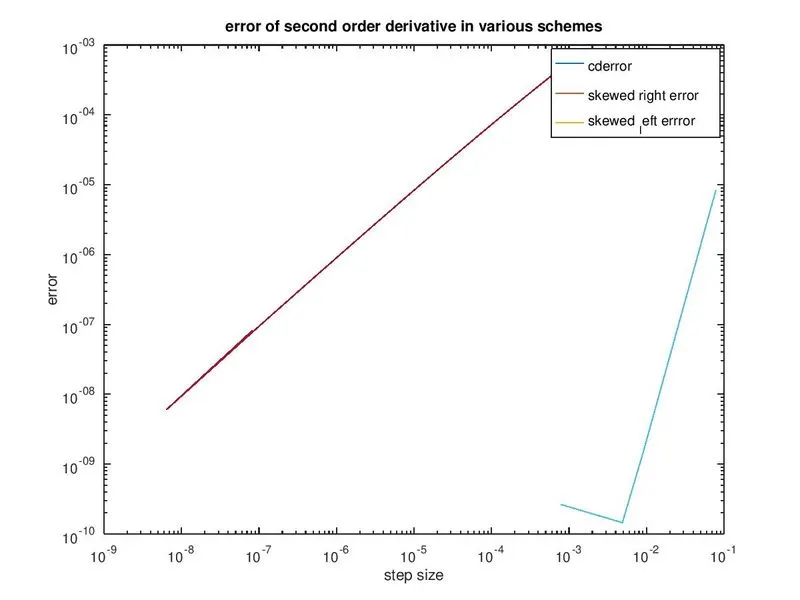
1. The Central Difference scheme has less error in comparison with skewed left and skewed right scheme
2. The skewed left and right schemes have same values for the chosen step size
3. The skewed scheme is suitable for boundaries where ,there are no nodes before or after the point at which approximation is required
4. Where as for central difference scheme requires a point before and after the chosen node where approximation is required.
5. Hence skewed right and skewed left are useful at boundary ,even though central difference can give higher approximation it is not suitable at boundaries