Week 7 - Simulation of a 1D Super-sonic nozzle flow simulation using Macormack Method
1D Quasi Sub Sonic to Super Sonic Nozzle
Symbols and notation
| `rho` | density |
| `rho_o` | reservoir density |
| `rho^'=(rho)/(rho_o)` |
dimensionless density |
| V | velocity |
| `V^'=V/(a_o)` | Dimension less velocity |
| `a_o` | sound velocity |
| T |
Temperature |
| `T_o` | Temperature of the reservoir |
| `T^'=T/T_o` | Dimensionless temperature |
| `t^'=(t)/(L/a_o)` | Dimension less time |
| `M =(V)/a_o` | Mach Number |
| L |
Length of the nozzle |
| P |
Pressure |
| `P'=P/P_o` |
pressure ratio |
| `A^'=A/A^star` |
Area ratio |
| `A^star` |
Throat area |
| `e` |
specific energy |
| F |
Flux terms |
| J |
Source terms |
The Nozzle is a device which increases the velocity at the expense of pressure, at the exit of the nozzle the velocity is higher in comparison with inlet velocity.
The process experienced by the fluid passing through the nozzle is called as expansion , which has a pressure drop. The thermodynamics process of this is expansion, if the nozzle is absolutely smooth and no friction effects are considered and the process is reversible we can assume the case is isentropic ,which is given by the relation
`P.V^(gamma) =constant` , where gamma is the ratio of specific heats ,for mono-atomic gases gamma value is 1.4
When a fluid is passed through the nozzle the velocity increases , Temperature decreases , Pressure decreases, Density decreases. these variation of variables will be shown in this project.
Since a nozzle is an open system we would be using the two approaches to solve the problem
- Conservative approach
- Non-Conservative approach
Firstly we need to know the governing equations which are required to solve this problem which are
- Continuity
- Momentum Equation
- Energy Equation
We would be extracting these three equations from the two approaches ,
Conservative Form
In an conservative form of approach , we asssume an infinitesimal element in space which is fixed , and mass is entering and leaving through it from its faces. Since the elemental volume is fixed , the mass changes due to the variation in the density . By using this approach the governing equations are generated , for further simplyfying these equation we use non dimensional parameters instead of dimensional one .
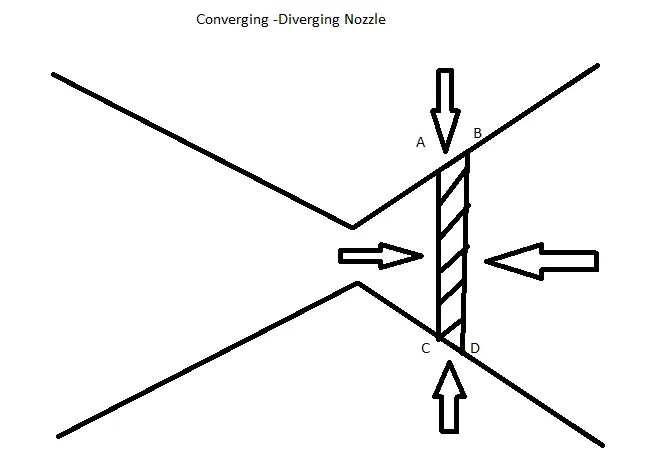
The above figure shows a conerging diverging nozzle , the cross section with smallest are is called throat , we can taken an infinitesimal element here ABCD which is fixed we will apply conservation of mass, momentum and energy on it to find the governing equations.
Our governing equations in the conservative form are
Continuity Equation
`(del rho^'.A^')/(delt) =(del rho^'.A^'.V^')/(delx)`
Momentum Equation
`(del rho^'.A^'.V^')/(delt) +((del rho^'.A^'.(V^')^2)+1/gamma*P^'.A^')/(delx)=1/gamma*P^'*((delA)/(delx))`'
Energy Equation
`del[(rho^'*((e')/(gamma-1)+gamma/2*(V')^2)*A^')]/(delt^')+del[(rho^'*((e')/(gamma-1)+gamma/2*(V')^2)*A^'*V^'+P^'A'V^')]/(delx^')`
these equations are converted in a compact form , without the primitive variables
`(delU_1)/(delt) =(delF_1)/(delx)`
`(delU_2)/(delt) =(delF_2)/(delx)+J_2`
`(delU_3)/(delt) =(delF_3)/(delx)`
where inturn the flux variables are in the form of of U's this form is called as pure form. This has an advantage of good stability in comparison with the primitve form
Non Conservative Form
In a non conservative approach the infinitesimal element is moving with the flow, as it moves the volume changes with changes in the density at different locations
The governing equations are in the form of
Continuity eqution
`(delrho')/(delt')=-rho'(delV')/(delx')-rho'V'(del(lnA'))/(delx')-rho(delV')/(delx)`
Momentum Equation
`(delV')/(delt')=-V'(delV')/(delx') -1/gamma*((delT')/(delx')+(T')/(rho')(delrho')/(delx'))`
Energy equation
`(delT')/(delt')=-V'(delT')/(delx') -(gamma-1)*T'((delV')/(delx')+(V')(del(lnA')/(delx'))``
Mc Cormack Scheme
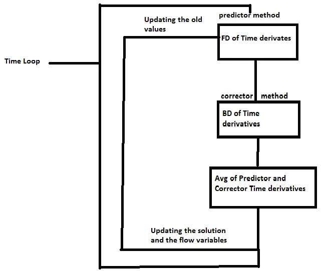
Using the above scheme the following code was written for both the approaches
 clear all
   clc
   close all
%no of nodes
n=31;
x = linspace(0,3,n);
dx = x(2)-x(1);
%grid size
rho_nc = 1-0.3146*(x);
%density intial values
t_nc = 1-0.2314*(x);
%temparature initial values
v_nc = (0.1+1.09.*x).*t_nc.^(0.5);
%velocity initial values
A = 1 + 2.2*(x - 1.5).^2;
% Area
gamma =1.4;
%ratio of specific heats
% no of time steps
C =0.5;
%Courant number
nt=1400;
%non conservative function
throat = (n+1)/2
[M_throat_n,rho_throat_n,t_throat,p_throat_n,Mach_n,v_n,rho_n,t_n,p_n,mass,k] = nonconservative(n,x,dx,nt,rho_nc,t_nc,v_nc,A,C,gamma,throat)
for i = 1:n
   a(i)= 1 + 2.2*(x (i)- 1.5).^2;
  if (x(i)>=1.5)
    rho(i) =0.634-0.3879*(x(i)-1.5);
    t(i) =0.833-0.3507*(x(i)-1.5);
     elseif(x(i)>0.5)
       rho(i)=1-0.366*(x(i)-0.5);
       t(i)=1-0.167*(x(i)-0.5);
     elseif (x(i)<=0.5)
       rho(i)=1;
       t(i)=1;
   endif
 endfor
 [M_th,rho_th,p_th,v_th,t_th,M_c,v,rho,t,p,k,u2]=conservative(n,nt,x,dx,rho,t,a,C,gamma,throat)
  figure(3)
  % velocity variation with time
  subplot(3,2,1)
  plot(x,v_n,"-b")
  hold on
  plot(x,v,"-r")
  legend("non conservative","conservative")
  title(sprintf(" Time step=%d",k))
  xlabel("x/L non dimensional length")
  ylabel("velocity")
  % density variation with time
  subplot(3,2,2)
  plot(x,rho_n,"-b")
  hold on
  plot(x,rho,"-r")
  legend("non conservative","conservative")
  xlabel("x/L non dimensional length")
  ylabel("density")
  % temparature variation with time
  subplot(3,2,3)
  plot(x,t_n,"-b")
  hold on
  plot(x,t,"-r")
  legend("non conservative","conservative")
  xlabel("x/L non dimensional length")
  ylabel("temparature")
  % pressure variation with time
  subplot(3,2,4)
  plot(x,p_n,"-b")
  hold on
  plot(x,p,"-r")
  legend("non conservative","conservative")
  xlabel("x/L non dimensional length")
  ylabel("pressure")
  % mass variation with time
  subplot(3,2,5)
  plot(x,mass,"-b")
  hold on
  plot(x,u2,"-r")
  legend("non conservative","conservative")
  xlabel("x/L non dimensional length")
  ylabel("Mass flow rate")

  % mach number variation with time
  subplot(3,2,6)
  plot(x,Mach_n,"-b")
  hold on
  plot(x,M_c,"-r")
  legend("non conservative","conservative")
  xlabel("x/L non dimensional length")
  ylabel("Mach number")


  % plots at the throat
  figure(4)
    k=1:1400;
   subplot(4,1,1)

  % density variation with time
  plot(k,rho_throat_n,"-b")
  hold on
  plot(k,rho_th,"-r")
  legend("non conservative","conservative")
  xlabel("time step")
  ylabel("density")

  % temparature variation with time
  subplot(4,1,2)
  plot(k,t_throat,"-b")
  hold on
  plot(k,t_th,"-r")
  legend("non conservative","conservative")
  xlabel("time step")
  ylabel("temparature")

  % pressure variation with time
  subplot(4,1,3)
  plot(k,p_throat_n,"-b")
  hold on
  plot(k,p_th,"-r")
  legend("non conservative","conservative")
  xlabel("time step")
  ylabel("pressure")

  % mach number variation with time
  subplot(4,1,4)
  plot(k,M_throat_n,"-b")
  hold on
  plot(k,M_th,"-r")
  legend("non conservative","conservative")
  xlabel("time step")
  ylabel("Mach number ")
The conservative function in this code
 function[M_th,rho_th,p_th,v_th,t_th,M_c,v,rho,t,p,k,u2]=conservative(n,nt,x,dx,rho,t,a,C,gamma,throat)
  u1= rho.*a;
  v =0.59./u1;
  u2 =rho.*a.*v;
  u3 = rho.*a.*((t./(gamma-1))+(0.5*gamma.*(v.^2)));
  dt =min((C.*dx)./(sqrt(t)+v))
  p =rho.*t;
  M_c =v./(sqrt(t));
  %%time step
 %%%%%%%%%%% time and space loop %%%%%%%%%%%%%%%%%%%%%%%%%
for k = 1:nt;
 p =rho.*t;
 dt =min((C.*dx)./(sqrt(t)+v))
##  dt =min((C.*dx)./(sqrt(t)+v))
  u1_old = u1;
  u2_old = u2;
  u3_old = u3;
  f1= u2;
  f2 = ((u2.^2)./u1) +((gamma-1)/gamma)*(u3-((gamma*0.5*(u2.^2))./u1));
  f3 =((gamma*u2.*u3)./u1) -(( gamma*(gamma-1)*0.5)*((u2.^3)./u1.^2));

  %% predictor step
 for i = 2:n-1;
 dadx(i) =(a(i+1)-a(i))/dx;

  %% continuity equation
  du1dt_p(i)  = -(f1(i+1)-f1(i))/dx;
  %% momentum equation
  %j2
  j2(i) = (1/gamma)*rho(i)*t(i)*dadx(i);
  du2dt_p(i) =  -((f2(i+1)-f2(i))/dx)+j2(i);
  %% Energy equation
  du3dt_p(i) =  -(f3(i+1)-f3(i))/dx;
 %%%
##  u2(1)=2*u2(2)-u2(3);
 u1(i) =u1(i)+du1dt_p(i)*dt;
 u2(i) =u2(i)+du2dt_p(i)*dt;
 u3(i) =u3(i)+du3dt_p(i)*dt ;
 endfor
 % updating the primitive variable and flux terms
       v = u2./u1;
       rho = u1./a;
      % temparature is updated by  using the values from the predictor
       t = (gamma-1)*((u3./u1)-(gamma*0.5*(v).^2));
      f1= u2;
  f2 = ((u2.^2)./u1) +((gamma-1)/gamma)*(u3-((gamma*0.5*(u2.^2))./u1));
  f3 =((gamma*u2.*u3)./u1) -(( gamma*(gamma-1)*0.5)*((u2.^3)./u1.^2));
%%% corrector method
 for j= 2:n-1;
   dadx(j) =(a(j)-a(j-1))/dx;;
   j2(j) = (1/gamma)*rho(j)*t(j)*dadx(j);
%% calculating the time difference of the pure form in corrector method
  %%continuty
  du1dt_c(j)  = -(f1(j)-f1(j-1))./dx;
  %%momentum
  du2dt_c(j) =  (-(f2(j)-f2(j-1))./dx) +j2(j);
  %%Energy
  du3dt_c(j) =  -(f3(j)-f3(j-1))./dx;
endfor
%%the final solution
 du1dt =(du1dt_c+du1dt_p)*0.5;
 du2dt =(du2dt_c+du2dt_p)*0.5;
 du3dt =(du3dt_c+du3dt_p)*0.5;
 % final solution update
 for l = 2:n-1;
    u1(l) =u1_old(l)+du1dt(l)*dt;
 u2(l) =u2_old(l)+du2dt(l)*dt;
 u3(l) =u3_old(l)+du3dt(l)*dt;
 endfor
 %outer time loop
 %%Applying the inlet boundary condition
   u1(1)=rho(1)*a(1);
   u2(1)=(2*u2(2))-u2(3);
   u3(1) =u1(1)*((t(1)/(gamma-1)+(gamma/2)*v(1)^2));
 %%Applying the exit boundary condition
 u1(n)=2*u1(n-1)-u1(n-2);
 u2(n)=2*u2(n-1)-u2(n-2);
 u3(n)=2*u3(n-1)-u3(n-2);
 %%Updation of the flow variables
    v = u2./u1;
    rho = u1./a;
    t = (gamma-1)*((u3./u1)-(gamma*0.5*(v).^2));
    p =rho.*t;
    M_c =v./sqrt(t);
    v_th=v(throat);
    rho_th(k) =rho(throat);
    t_th(k) = t(throat);
    M_th(k) =M_c(throat);
    p_th(k) =p(throat);
    w = 0.579.*ones(1,n);
  figure(2)
  if (k==50)
    plot(x,u2)
    hold on
    elseif (k==100)
    plot(x,u2)
    hold on
    elseif (k==150)
    plot(x,u2)
    hold on
    elseif (k==200)
    plot(x,u2)
    hold on
    elseif (k==500)
    plot(x,u2)
    hold on
    elseif (k==700)
    plot(x,u2)
    hold on
    elseif (k==1400)
    plot(x,u2)
    hold on
    plot(x,w)
    legend({"50 DeltaT","100 DeltaT","150 DeltaT","200 DeltaT","500 DeltaT","700 DeltaT","1400 DeltaT","Analytical"})
  endif
  xlabel("x/L non dimensional length")
  ylabel("mass flow rate --rho.a.v/((rho_o).(a_o).(v_o))")
  title("time wise variation of the mass flow rate in conservative ")
 endfor
 endfunction
Function for non conservative form
function [M_throat_n,rho_throat_n,t_throat,p_throat_n,Mach_n,v_n,rho_n,t_n,p_n,mass,k]=nonconservative(n,x,dx,nt,rho_n,t_n,v_n,A,C,gamma,throat)
for k =1:nt;
    p_n =rho_n.*t_n;
    rho_old=rho_n;
    t_old=t_n;
    v_old=v_n;
    dt =min(C*(dx./(sqrt(t_n)+v_n)));
     mass=rho_n.*A.*v_n;
    %clf
  %predictor method
  for j = 2:n-1;
    dvdx =(v_n(j+1) -v_n(j))/dx;
    drhodx =(rho_n(j+1) -rho_n(j))/dx;
    dtdx =(t_n(j+1) -t_n(j))/dx;
    dlogdx = (log(A(j+1))-log(A(j)))/dx;
    drhodt_p(j) = -rho_n(j)*(dvdx) -(rho_n(j)*v_n(j))*(dlogdx) -v_n(j)*(drhodx);
    dvdt_p(j) = -v_n(j)*(dvdx) -((dtdx + (t_n(j)/rho_n(j))*drhodx)/gamma);
    dTdt_p(j)=-v_n(j)*dtdx -(gamma-1)*t_n(j)*(dvdx+(v_n(j)*dlogdx));
     v_n(j)= v_n(j)+dvdt_p(j)*(dt);
     t_n(j)=t_n(j)+dTdt_p(j)*(dt);
     rho_n(j) =rho_n(j)+drhodt_p(j)*(dt);
  endfor
  %corrector method
  for j = 2:n-1;
    dvdx =(v_n(j) -v_n(j-1))/dx;
    drhodx =(rho_n(j) -rho_n(j-1))/dx;
    dtdx =(t_n(j) -t_n(j-1))/dx;
    dlogdx = (log(A(j))-log(A(j-1)))/dx;
    drhodt_c(j) = -rho_n(j)*(dvdx) -(rho_n(j)*v_n(j))*(dlogdx) -v_n(j)*(drhodx);
    dvdt_c(j) = -v_n(j)*(dvdx) -((dtdx + (t_n(j)/rho_n(j))*drhodx)/gamma);
    dTdt_c(j)=-v_n(j)*dtdx -(gamma-1)*t_n(j)*(dvdx+(v_n(j)*dlogdx));
     v_n(j)= v_n(j)+dvdt_c(j)*(dt);
     t_n(j)=t_n(j)+dTdt_c(j)*(dt);
     rho_n(j) =rho_n(j)+drhodt_c(j)*(dt);
  endfor
   % final solution
  drhodt =(drhodt_c+drhodt_p)*0.5;
  dvdt =(dvdt_c+dvdt_p)*0.5;
  dTdt =(dTdt_c+dTdt_p)*0.5;
  for i =2:n-1;
    %
     v_n(i)= v_old(i)+dvdt(i)*(dt);
     t_n(i)=t_old(i)+dTdt(i)*(dt);
     rho_n(i) =rho_old(i)+drhodt(i)*(dt);
     p_n(i) =rho_n(i)*t_n(i);
  endfor
  %initial conditions
  v_n(1) =2*v_n(2)-v_n(3);
  %final conditions
  v_n(n) =2*v_n(n-1)-v_n(n-2);
  rho_n(n) = 2*rho_n(n-1)-rho_n(n-2);
  t_n(n) =2*t_n(n-1)-t_n(n-2);
  M_throat_n(k) = v_n(throat)/sqrt(t_n(throat));
  rho_throat_n(k)=rho_n(throat);
  p_throat_n(k)=p_n(throat);
  Mach_n =v_n./sqrt(t_n);
  t_throat(k) =t_n(throat);
  u2 = rho_n.*A.*v_n;
  mass= u2;
  w =0.579.*ones(1,n);
  %plotting the variation of mass flow rate for various timesteps in non conservative form
 figure(1)
  if (k==50)
    plot(x,u2)
    hold on
    elseif (k==100)
    plot(x,u2)
    hold on
    elseif (k==150)
    plot(x,u2)
    hold on
    elseif (k==200)
    plot(x,u2)
    hold on
    elseif (k==500)
    plot(x,u2)
    hold on
    elseif (k==700)
    plot(x,u2)
    hold on
    elseif (k==1400)
    plot(x,u2)
    hold on
    plot(x,w)
    hold on
    legend({"50 DeltaT","100 DeltaT","150 DeltaT","200 DeltaT","500 DeltaT","700 DeltaT","1400 DeltaT","Analytical"})
  endif

  xlabel("x/L non dimensional length")
  ylabel("mass flow rate --rho.a.v/((rho_o).(a_o).(v_o))")
  title("time wise variation of the massflow rate non conservative")
   endfor
endfunction
Steady State Results
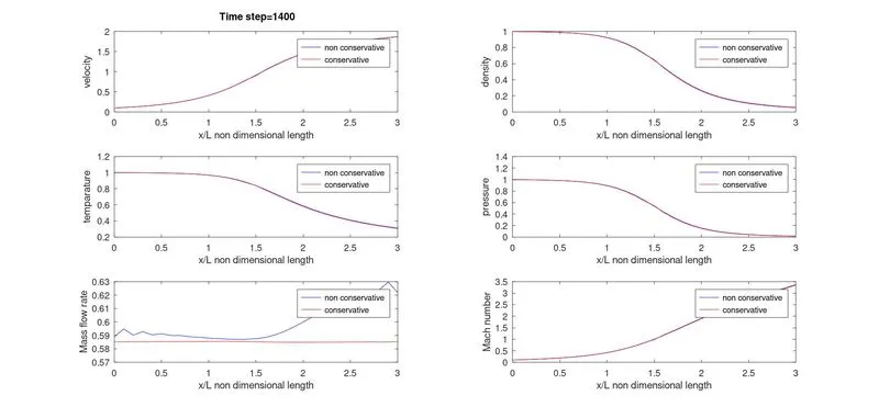
In the above figure
It is observed that conservation form of the equation the mass flow is captured to a great extent in comparison to the non conservative form
The steady state mass distribution in the conservative form is much closer to the analytical value which is 0.579
Conservation form deals with better mass flow distribution
Non conservation form has lower residuals , since the amount at which residuals decays dictates the quality of the algorithm used , is called the
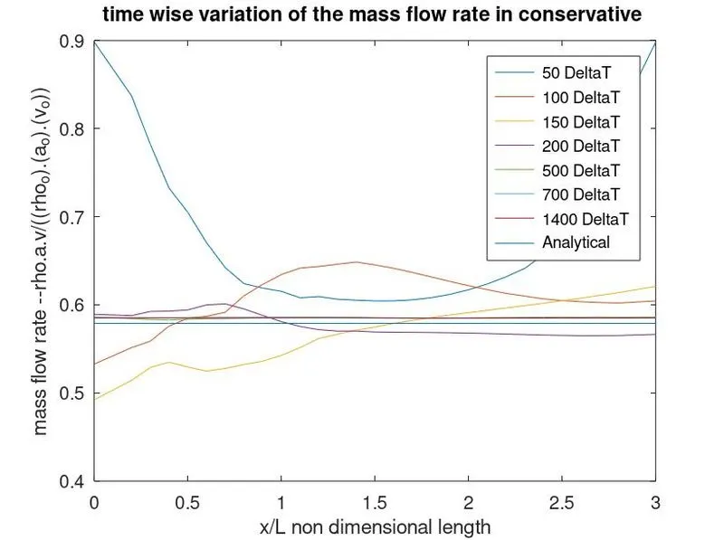
conservative form shows the better variation with respect to time , it also shows that after 700 time steps the solution reaches the steady state and closely matches with the anlaytical mass flow rate which 0.579
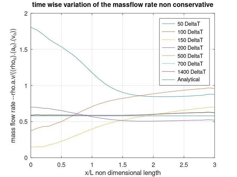
In non conservative form it shows that after 700 time steps the solution reaches the steady state and closely matches with the anlaytical mass flow rate which 0.579
Variation of the NonDimensional Parameters at throat
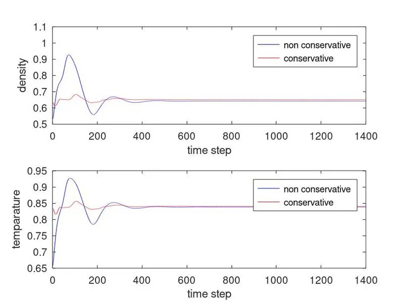
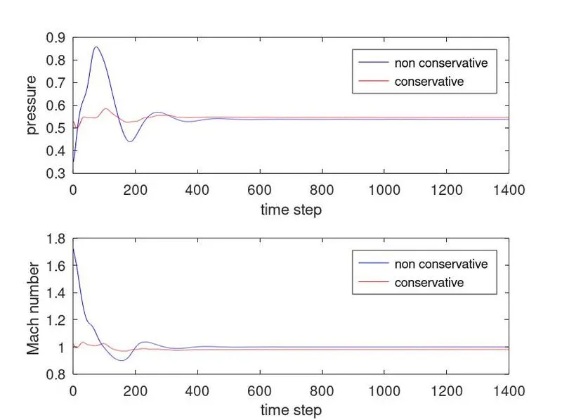
From the above plots we observe that the paramters at initial time steps are changing rapidly hence the solution also changes rapidly in the later stages the variation is reduces so does the changes in the solution
Grid Independece test
| grid points | `rho/rho_o` | `T/T_o` | `P/P_o` | `M` | |
|
case 1 conservative |
31 | 0.6504 | 0.84 | 0.5464 | 0.9817 |
|
case 2 non conservative |
31 | 0.6421 | 0.838 | 0.5381 | 0.9995 |
|
case 1 conservative |
61 | 0.6382 | 0.8352 | 0.5330 | 0.9993 |
|
case 2 non conservative |
61 | 0.6394 | 0.8362 | 0.5347 | 0.9997 |
| exact |
analytical |
0.634 | 0.833 | 0.528 | 1 |
The above table is steady state comparison of the conservative and non conservative form with increasing the grid points its observed that the non conservative form is closer to the exact solution .