Week-11 Challenge: Braking

1) According to the need a driving cycle is created for 350 secs with variable speed.

After creating the data in the excel sheet, its being plotted in speed vs time graph

Then any two instances from the drive cycle is taken and the braking energy for those individual instance is calculated using the formula -

Braking energy = 0.5*mass*(Vf - Vi)^2

where

Vf - final velocity

Vi = intial velocity

let mass = 2000kg

from the driving cycle

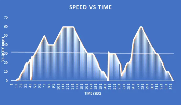
braking point 1 = 60 mps to 40 mps

Braking energy 1 = 0.5*2000*(40-60)^2 = 400kJ

braking point 2 = 40 mps to 0 mps

Braking energy 2 = 0.5*2000*(0-40)^2 = 800kJ

Total braking energy = Braking energy 1 + Braking energy 2 = 1200kJ

2)

Electric Motor Braking

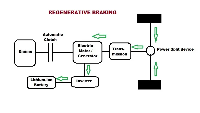
The electric motor braking is also known as Regenerative Braking, which is an energy recovery mechanism that slows down a moving vehicle or object by converting its kinetic energy into a form that can be either used immediately or stored until needed.

When we press the brake pedal, we cut off the power supply to the motor and now the motor will be in rotation due to its inertia. As this rotation is happening inside the magnetic field, a back emf is generated which produces a negative torque and that is used as the brakes to reduce the vehicle speed. Also the current flows in reverse direction, using a bi-directional inverter, we can store the current back into the battery. This process of braking by the effect of negative torque produced and where the motor acts as a generator in producing the current out of the motor’s rotation and storing it back into the battery is called Regenerative braking.

Speed and Torque characteristics of a DC Motor

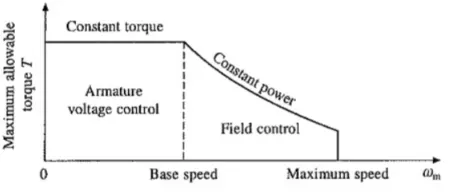
From the above figure, we can see the speed and torque behaviour of an electric motor.

During the initial low speed, the torque is high and this is the constant torque region. As speed builds up after the critical speed point, the torque gradually decreases and this is known as constant power region.

So during high speeds, the motor will be at constant power region and while braking, due to high speed of the motor, the negative torque produced will be less.

But while starting the motor, the speed will be very less and at this stage, the motor will be operating in constant torque region and this is the reason for high accelerating torque during the start of motor.

From this, we can say that the braking torque produced at high speed motor operations will be lesser than the starting torque of an electric motor. Also there are other reasons like battery limitations due to which we cannot get high braking torque. The rate of discharge is always higher than the rate of charging due to the battery’s chemical compositions.

Combination of Electric and Mechanical brakes

Motor of electric vehicle is able to be used to brake regeneratively, so braking energy can be recycled.

Braking stability of electric vehicles with electro-hydraulic hybrid braking system can be influenced by braking force distribution between hydraulic braking force and regenerative braking force.

Electric cars have regenerative braking and this does substantially reduce the need for hydraulic braking. But there are limitations like, the maximum deceleration with the engine alone is far smaller than with brake assistance. Hence, an ordinary frictional brake system is needed to make the car stop instantly if required.

When the regenerative capacity is less than the actual braking required, mechanical brakes are applied at those times.

Brake control strategy

When the brake control is pressed, the control signal is sent to both the hydraulic cylinder and power converters for producing both Frictional braking and Regenerative braking.

Brake System of EVs and HEVs

1. Series Brake — Optimal Feel
2. Series Brake — Optimal Energy Recovery
3. Parallel Brake
4. Antilock Brake System (ABS)

There are two ways of applying the combination of brakes and they are classified as

1. Series – The regenerative braking and frictional braking are applied one after another.
2. Parallel - The regenerative braking and frictional braking are applied at the same time.

The series braking and parallel braking is chosen based on two parameters, one is Driver’s comfort and other one is based on the Efficiency.

The parallel combined braking technology is further developed as EDIB, which is Electric Driven Intelligent Braking.

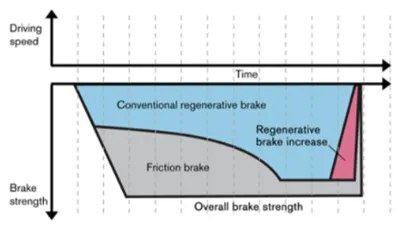
EDIB Technology

The above figure shows the Electric Driven Intelligent Braking system, where both the Regenerative brakes and Frictional brakes are applied at the same time.

After braking, the speed reduces from higher speed values and at this moment, the percentage of composition if the combined braking changes. So after brake application, the speed is reduced to lower values. Here torque will be high and the motor will be operating at constant torque region. Now at this point, the percentage of frictional brake application is reduced and regenerative braking is increased because at this point, more negative torque can be generated and thus higher electric power generated out of this braking can also be fed back to the battery. Hence, using this technology in braking, an electric vehicle certainly increases the stopping power and also contributes to higher efficiency figures.

3)

• First of all an array of data is being created for time and speed.
• The constants for copper, iron, windage and constant loss are being defined.
• Equation for all the losses and input power is implemented
• The efficiency of the system is being calculated.
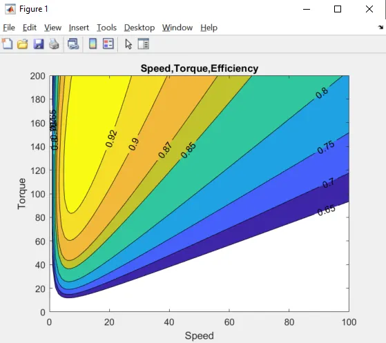
• Then using all the above data a contoured graph has been generated.

clear all
close all
clc
%% defining array of data for time and speed

time = linspace(0,500);
speed = linspace(0,150);

%% defining the different constants

kc = 0.5;
ki = 0.005;
kw = 0.00001;
const = 20;

[T,S] = meshgrid(time,speed);

%% implementing the various required equations

output_power = (T.*S);
cu_loss = (T.^2)*kc;
iron_loss = S*ki;
windage_loss = (S.^3)*kw;

input_power = output_power + cu_loss + iron_loss + windage_loss + const;

efficiency = output_power./input_power;

%% contouring of the data

X = [0.65,0.70,0.75,0.80,0.85,0.87,0.90,0.92,0.95];
box off
grid off
[C,h] = contourf(T,S,efficiency,X);
clabel(C,h,'labelspacing',500);
%plot(time,speed);
xlabel('Speed');
ylabel('Torque');
title('Speed,Torque,Efficiency');

the output is shown below