Final Project: Electric Rickshaw modelling
AIM - To create MATLAB model of an electric rickshaw
Block diagram of the MATLAB model
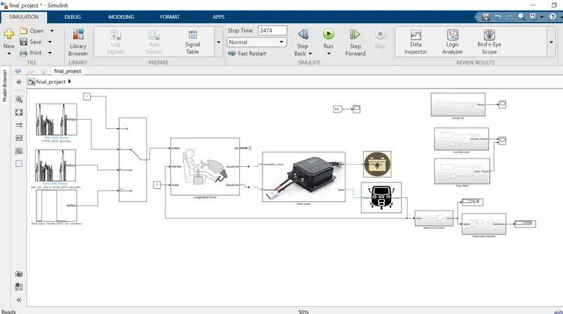
Now discussing each components of the model in brief
1) Drive cycle
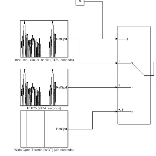
Three different drive cycle have been chosen for the simulation along with a custom made one
using the multiport switch
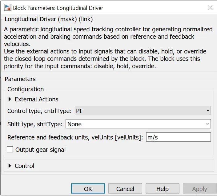
Next component is logitude driver
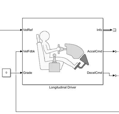
A parametric longitudinal speed tracking controller for generating normalized acceleration and braking commands based on reference and feedback velocities.
Use the external actions to input signals that can disable, hold, or override the closed-loop commands determined by the block.
The Longitudinal Driver block implements a longitudinal speed-tracking controller. Based on reference and feedback velocities, the block generates normalized acceleration and braking commands that can vary from 0 through 1. You can use the block to model the dynamic response of a driver or to generate the commands necessary to track a longitudinal drive cycle
settings used
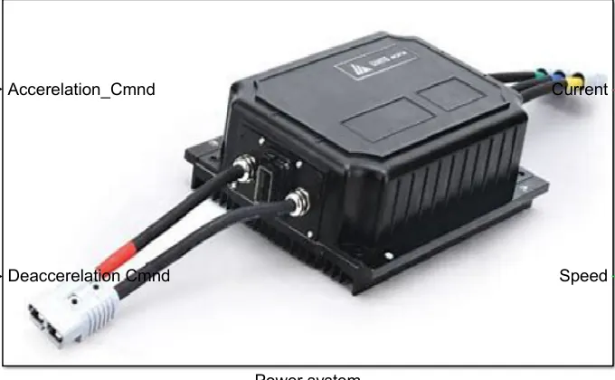
Next component is the combination of power supply and motor control
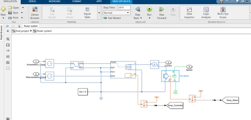
PWM
Pulse Width Modulation (PWM) is a nifty current control technique that enables you to control the speed of motors, heat output of heaters, and much more in an energy-efficient (and usually quieter) manner. Existing applications for PWM include, but are not limited to:
- Variable speed fan controllers.
- VRF HVAC compressor drives.
- Hybrid and electric vehicle motor drive circuits.
- LED Dimmers.
Pulse width modulation has changed the world by slashing the power consumption of appliances utilizing motors such as inverter air conditioners [PDF], inverter refrigerators, inverter washing machines, among many others. For example, inverter air conditioners can consume less than half the energy that their non-inverter counterparts do in some cases.
In this day and age, if a device is advertised as having a variable speed compressor or variable speed fan (this doesn’t include two or three-speed fans), there is a significant chance that it is utilizing PWM!
Why Use PWM?
Aspiring electrical engineers may want to know why they should use pulse width modulation to control devices, and homeowners have similar question which has the same answer: Why use inverter air conditioners, or other variable speed appliances?
The answer to both questions is: PWM varies the speed of the appliances’ motors so they only consume as much power as they need, but without the usual consequence of burning off unused current as heat. An example of an older alternative is a simple transistor circuit that varies the current passing through it by varying its resistance.
The same efficiency rule that applies to resistors also applies to transistors — Their resistance results in wasted energy because they burn off some of it as heat. They act like heaters in that regard.
Fortunately, these circuits were never mainstream. Appliances such as air conditioners and refrigerators just ran at full speed all the time, making lots of noise, and wasting lots of energy because they had to cycle on and off frequently.
PWM does make use of transistors, but in a different way, as explained below.
PWM Motor Controller Example.
If you’re looking to get started with PWM, a great entry point would be a 555 PWM circuit, Arduino PWM circuit (very convenient, as you can easily modify its behaviour via a simple source code modification), or the MSP30 PWM circuit that I wrote about on Kompulsa.
How Does PWM Work?
PWM works by pulsating DC current, and varying the amount of time that each pulse stays ‘on’ to control the amount of current that flows to a device such as an LED. PWM is digital, which means that it has two states: on and off (which correspond to 1 and 0 in the binary context, which will become more relevant to you if using microcontrollers).
The longer each pulse is on, the brighter the LED will be. Due to the fact that the interval between pulses is so brief, the LED doesn’t actually turn off. In other words, the LED’s power source switches on and off so fast (thousands of times per second) that the LED actually stays on without flickering. This is called PWM dimming, and such as circuit is just called a PWM LED dimmer circuit.
The squares in the PWM illustration below are the pulses which represent ‘on’ time, and the depressed areas represent the time that the power is ‘off’. Both the squares and depressed areas are the same ‘width’, therefore the duty cycle is 50%. PWM signals are typically square waves, like the one in the illustration below.

A PWM signal (square wave) with a 50% duty cycle.
If the duty cycle of a PWM power supply is set to 70%, then the pulse is on for 70% of the time, and it is off 30% of the time. Duty cycle refers the amount of time it is on. At a 70% duty cycle, an LED’s brightness should be near 70%. The correlation between duty cycle and brightness is not 100% linear, as the efficiency of LEDs varies with the amount of current supplied.
If the duty cycle was 0%, the entire signal would be flat, as shown below. A PWM duty cycle of 0% means that the power is off. In such a state, an LED would not be operational. It would simply be off.

PWM signal (square wave) with a duty cycle of 0%. This means the power is off.
The key reason that PWM circuits are so efficient is that they don’t try to partially restrict the flow of current using resistance. They turn the current fully on and fully off. They just vary the amount of time that it is on instead.
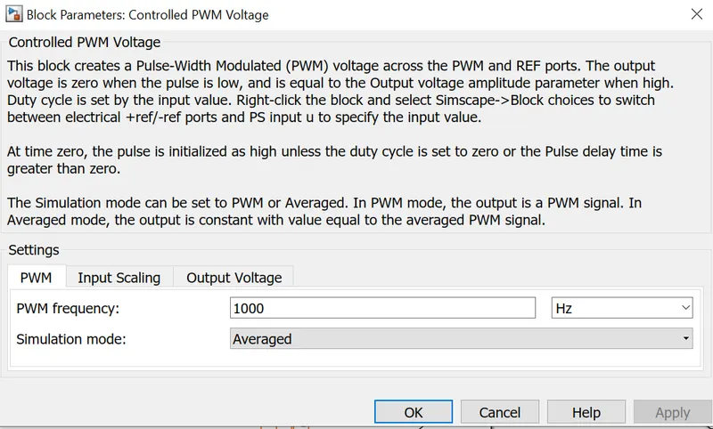
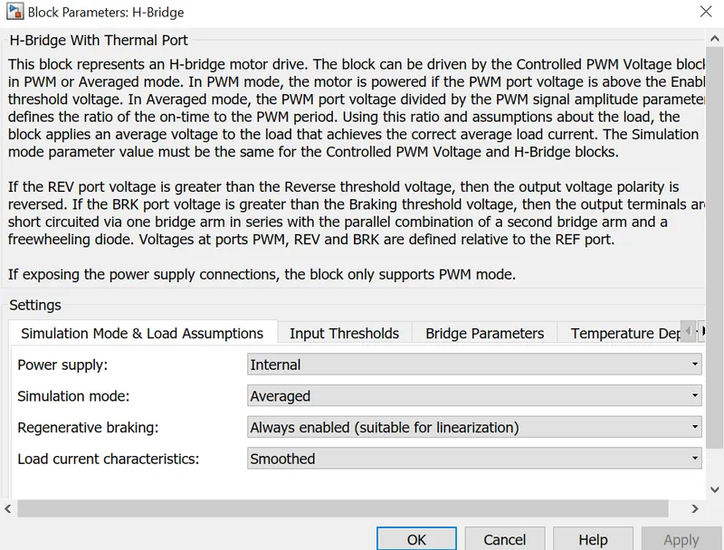
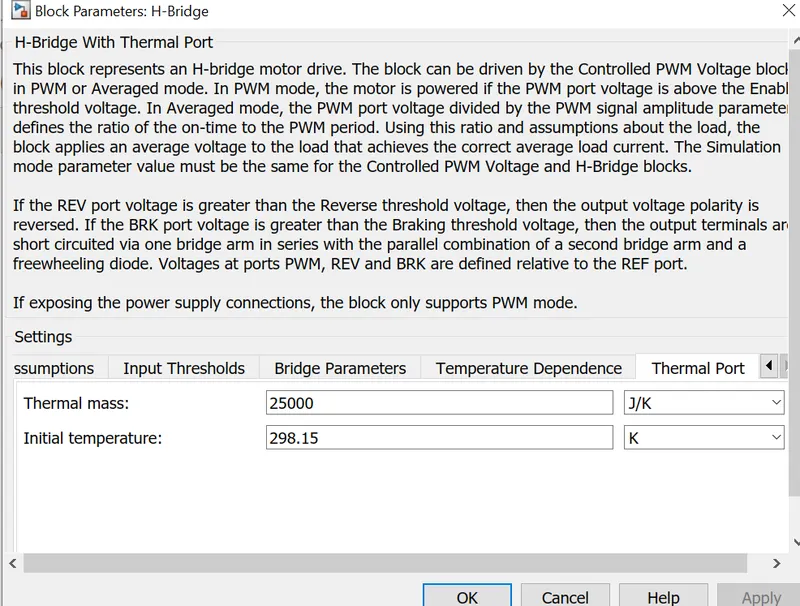
SETTINGS USED HERE ARE
H BRIDGE
In general an H-bridge is a rather simple circuit, containing four switching element, with the load at the center, in an H-like configuration:

The switching elements (Q1..Q4) are usually bi-polar or FET transistors, in some high-voltage applications IGBTs. Integrated solutions also exist but whether the switching elements are integrated with their control circuits or not is not relevant for the most part for this discussion. The diodes (D1..D4) are called catch diodes and are usually of a Schottky type.
The top-end of the bridge is connected to a power supply (battery for example) and the bottom-end is grounded.
In general all four switching elements can be turned on and off independently, though there are some obvious restrictions.
Though the load can in theory be anything you want, by far the most pervasive application if H-bridges is with a brushed DC or bipolar stepper motor (steppers need two H-bridges per motor) load. In the following I will concentrate on applications as a brushed DC motor driver.
Static Operation
The basic operating mode of an H-bridge is fairly simple: if Q1 and Q4 are turned on, the left lead of the motor will be connected to the power supply, while the right lead is connected to ground. Current starts flowing through the motor which energizes the motor in (let’s say) the forward direction and the motor shaft starts spinning.

If Q2 and Q3 are turned on, the reverse will happen, the motor gets energized in the reverse direction, and the shaft will start spinning backwards.

In a bridge, you should never ever close both Q1 and Q2 (or Q3 and Q4) at the same time. If you did that, you just have created a really low-resistance path between power and GND, effectively short-circuiting your power supply. This condition is called ‘shoot-through’ and is an almost guaranteed way to quickly destroy your bridge, or something else in your circuit.

PMDC motor
Definition: It is a type of motor similar to that of a normal motor but the difference is it has no field coil. It generates torque by the interaction of armature flux and permanent flux. The armature of this type of motor is shown in the figure below.
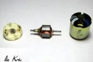
Disassembled Motor
Construction
It consists of a frame in which the inner peripherals of the motor are inserted. It acts as a protected shield to the motor. The frame is of a cylindrical shape made of silicon steel to avoid losses. The permanent magnets are placed inside the cylindrical tube which acts as a stator. The moving section consists of armature core and bearings. The armature core includes commutator and brushes. The armature core consists of some slots in which the armature winding is housed. The commutator acts as a converting device and brushes are used to supply the current to the commutator. The DC supply is applied to the armature by connecting the terminals to the brushes.
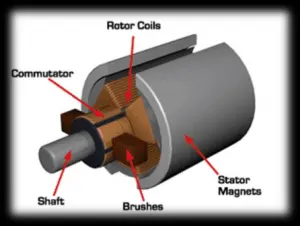
Working
The working of this type is similar to that of a normal DC motor. It runs approaching the origin of Electromagnetic Induction. Here the magnetic induction occurs between the armature field flux and permanent magnet field flux. Due to the interaction of these fluxes, a torque is developed. Let us discuss in detail how this torque is developed.
We know that according to the Lorentz force equation a current-carrying conductor placed in a magnetic field exhibits a force in a particular direction. In view of this statement, in this motor, the armature core is set below the impact of a permanent magnetic field and given a DC supply. Due to this, the current starts to flow in the armature winding and the coil gets energized. At this time, as these current-carrying coils are under the magnetic field a force is exhibited on these coils. This force tends to move the coil in a particular direction. Fleming’s Left-hand rule is used to know the movement. Accordingly, the coils exhibit some force in a particular direction and tend to rotate.
PMDC characteristics
The voltage equation of this type of motor is given by
V = Kt w + IR + L dI/dt
At steady-state condition, the current is considered as zero, then dI/dt = 0. The final equation that we get is V = Kt w + IR.
The equation in terms of w rad/sec keeping torque constant we get
W = V / Kt – R/ Kt2 Ƭ
The above equation determines the relation between torque and speed. From this, we can draw the curve between torque and speed.
The curve drawn between torque and speed is explained as below.
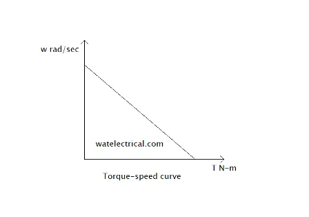
Speed Torque Curve
W = V / Kt gives the no-load speed of the motor.
Speed Control of PMDC Motor
The speed control of a normal motor can be done by either varying the field flux in series with armature or by varying the voltage applied. But in this motor, as a field winding is not in series with its armature it can be controlled by varying the voltage applied.
We know that in DC motor
E α φ N
E α φ N
T α Ia φ
T α Ia
V = E + Ia Ra
V = KN + Ia Ra
N = V – Ia Ra / K
In permanent magnet type, as the field is constant we can omit flux. The armature has some resistance which can be varied. Hence, by varying resistance and voltage speed of this motor can be controlled.
The difference between the winding diagram of a normal and this motor is explained.
Advantages
- Highly efficient
- Loss of power losses
- Smaller size
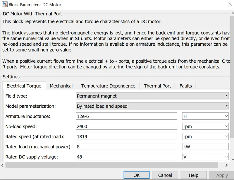
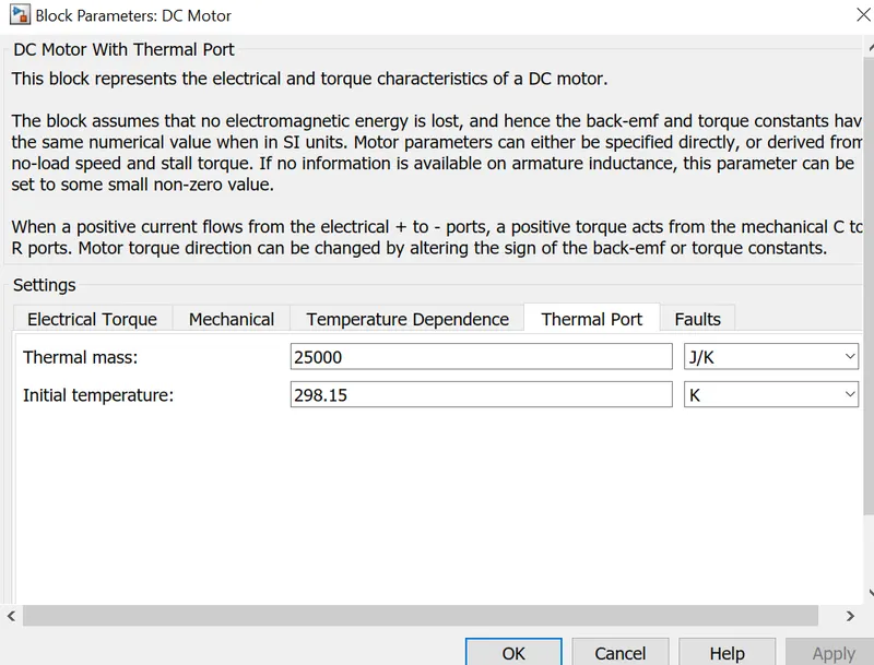
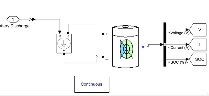
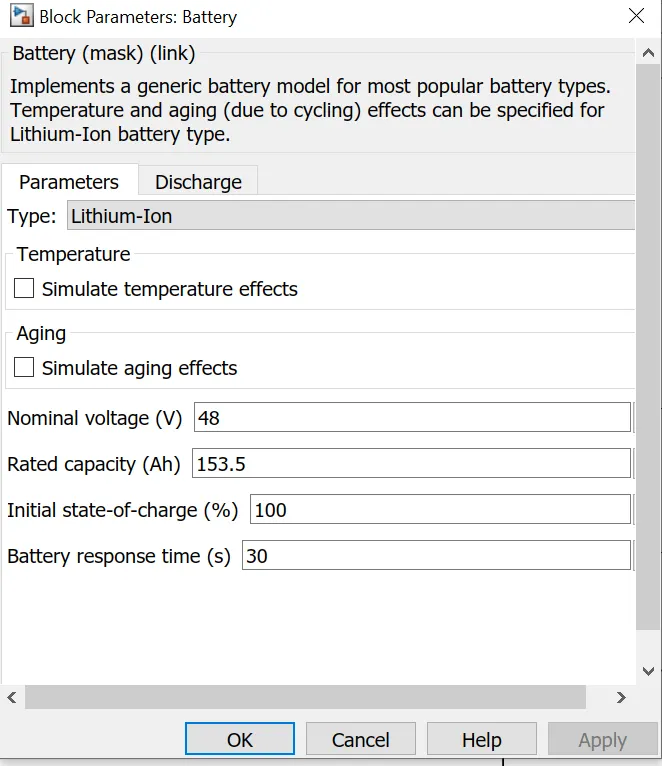
BATTERY MODULE
THE INTERNAL OF THE BATTERY SUBSYSTEM
Lithium-ion batteries power the lives of millions of people each day. From laptops and cell phones to hybrids and electric cars, this technology is growing in popularity due to its light weight, high energy density, and ability to recharge.
So how does it work?
This animation walks you through the process.
THE BASICS
A battery is made up of an anode, cathode, separator, electrolyte, and two current collectors (positive and negative). The anode and cathode store the lithium. The electrolyte carries positively charged lithium ions from the anode to the cathode and vice versa through the separator. The movement of the lithium ions creates free electrons in the anode which creates a charge at the positive current collector. The electrical current then flows from the current collector through a device being powered (cell phone, computer, etc.) to the negative current collector. The separator blocks the flow of electrons inside the battery.
CHARGE/DISCHARGE
While the battery is discharging and providing an electric current, the anode releases lithium ions to the cathode, generating a flow of electrons from one side to the other. When plugging in the device, the opposite happens: Lithium ions are released by the cathode and received by the anode.
ENERGY DENSITY VS. POWER DENSITY
The two most common concepts associated with batteries are energy density and power density. Energy density is measured in watt-hours per kilogram (Wh/kg) and is the amount of energy the battery can store with respect to its mass. Power density is measured in watts per kilogram (W/kg) and is the amount of power that can be generated by the battery with respect to its mass. To draw a clearer picture, think of draining a pool. Energy density is similar to the size of the pool, while power density is comparable to draining the pool as quickly as possible.
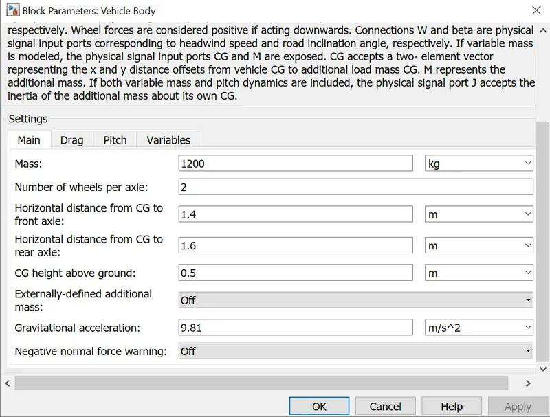
VEHICAL BODY SUBSYSTEM
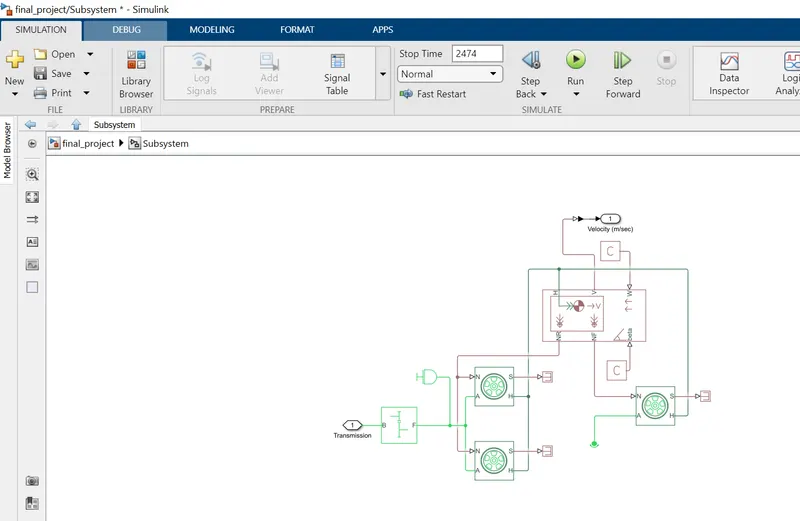
Represents a two-axle vehicle body in longitudinal motion. The block accounts for body mass, aerodynamic drag, road incline, and weight distribution between axles due to acceleration and road profile. The vehicle can have the same or a different number of wheels on each axle. Optionally include pitch and suspension dynamics or additional variable mass and inertia. The vehicle does not move vertically relative to the ground.
Connection H is the mechanical translational conserving port associated with the horizontal motion of the vehicle body. The resulting traction motion developed by tires should be connected to this port. Connections V, NF, and NR are physical signal output ports for vehicle velocity and front and rear normal wheel forces, respectively. Wheel forces are considered positive if acting downwards. Connections W and beta are physical signal input ports corresponding to headwind speed and road inclination angle, respectively. If variable mass is modeled, the physical signal input ports CG and M are exposed. CG accepts a two- element vector representing the x and y distance offsets from vehicle CG to additional load mass CG. M represents the additional mass. If both variable mass and pitch dynamics are included, the physical signal port J accepts the inertia of the additional mass about its own CG
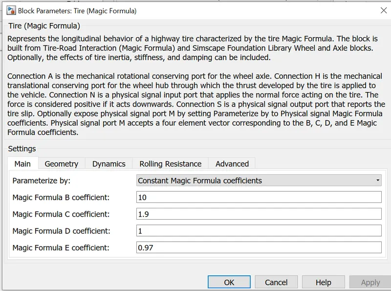
The block is built from Tire-Road Interaction (Magic Formula) and Simscape Foundation Library Wheel and Axle blocks. Optionally, the effects of tire inertia, stiffness, and damping can be included.
Connection A is the mechanical rotational conserving port for the wheel axle. Connection H is the mechanical translational conserving port for the wheel hub through which the thrust developed by the tire is applied to the vehicle. Connection N is a physical signal input port that applies the normal force acting on the tire. The force is considered positive if it acts downwards. Connection S is a physical signal output port that reports the tire slip. Optionally expose physical signal port M by setting Parameterize by to Physical signal Magic Formula coefficients.
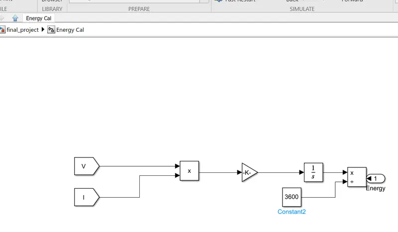
THE ENERGY CALULATION BLOCKS ARE
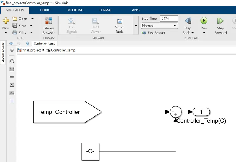
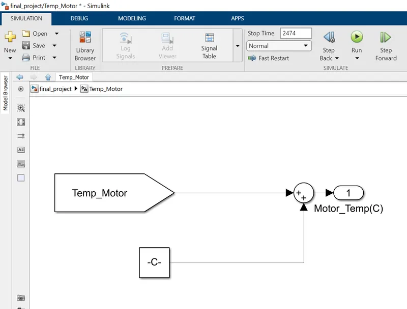
GETTING THE TEMPERATURE OF MOTOR AND CONTROLLER
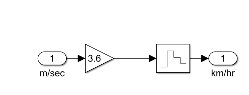
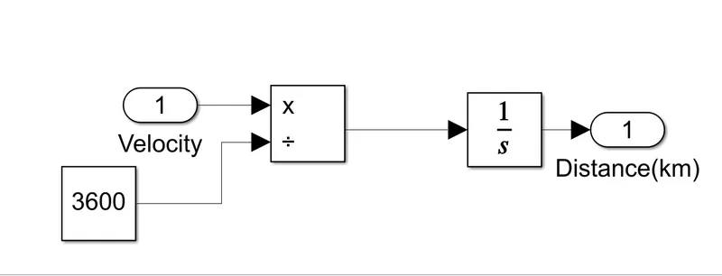
SUBSYSTEM FOR DISTANCE CALCULATION
RESULTS OBTAINED ARE
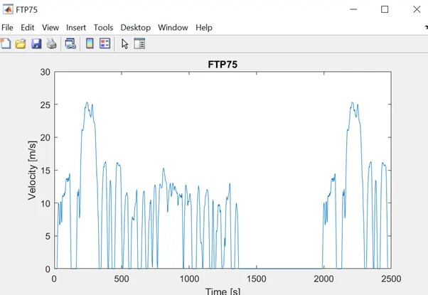
DRIVE CYCLE
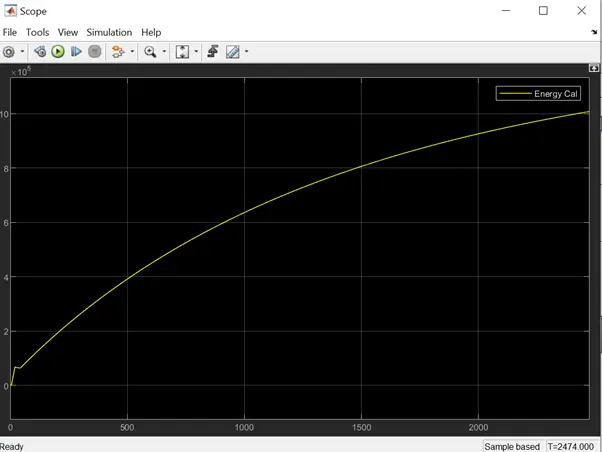
ENERGY GRAPH
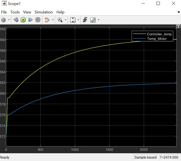
TEMPERATURE DATA FOR BOTH THE MOTOR AND CONTROLLER
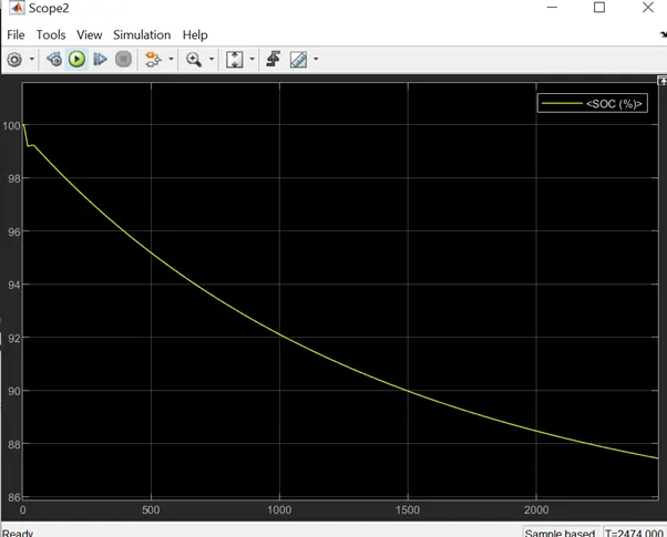
DISCHARGE GRAPH FOR THE BATTERY