Week 7 State of charge estimation

1) Simulate the 3 test cases from harness dashboard

Step 1) opening the dashboard

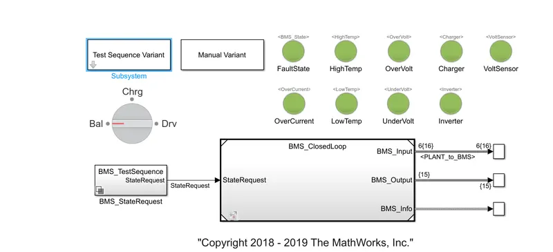
2 - select the first test 1 sequence we can see the sequence pattern

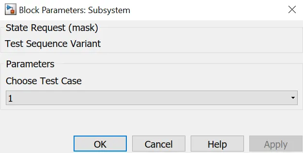
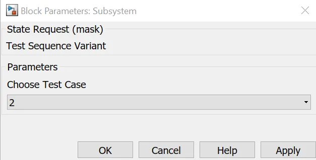
3- from the BMS state request, we can select test

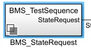
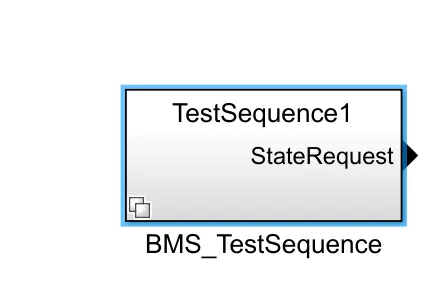
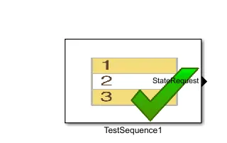
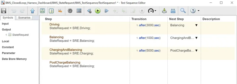
When simulation will start. the model will be in driving condition.

After 3000 seconds it will be in standby mode

After 1000 seconds it will be in charging mode followed by 4000 sec of charging

When we run the simulation. the indicators in the model will show errors if there is any.

Results

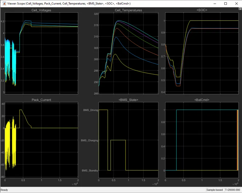
1) First plot shows us the cell voltages which is fluctuating between 3.2 and 3.7 V between 0 and 3000 seconds. It indicates that the nominal voltage was 3.7 and it decreased to 3.2 per cell.

2) During the charging phase it rises to 4.2 V (between 4000 to 9000 seconds).

3) When BMS will be in standby mode the voltages will not be reduced.

4) As the battery discharges while driving. it is displayed in the legative direction (till -60A).

5) Current rises to 30A during charging and then drops to 0 during standby.

6) Third plot shows the trend of the battery pack's cell temperatures. which range from 290K to 315K. The temperature of the cells rises during battery depletion and temperature of the cells reduces during charging and standby mode.

7) As the sixth cell has the highest temperature which indicates that it is discharged the most.

8) The BMS states are depicted in the fourth plot. As previously stated. the driving time ranged from 0 to 3000 seconds. the charging time unged from 4000 to 9000 seconds. and the standby time ranged from 9000 to 20000 seconds.

9) The SOC rapidly decreases to 0.45 during driving and fully charging back to 100% charging. In standby mode.

10) From the sixth cell of the battery pack to the first cell. the balancing of cells is resented in descending sequence.

case 2)

Results

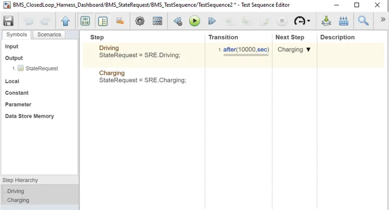
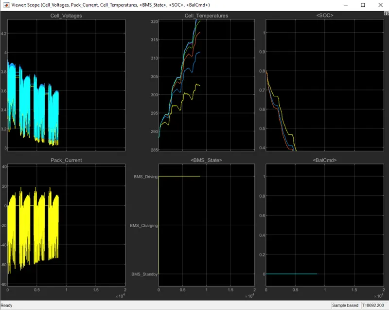
1) in driving mode until the battery pack's SOC is depleted.

2) The battery pack lasts only 8960 seconds on a single charge. There is no charging or standby mode in this test sequence.

3) The voltages range from 3.7 to 3V where 3V is the individual cell's cutoff voltage.

4) The battery pack can discharge up to its maximum capacity which is 60A .

5) The temperature of the cells continues to rise as a result of the constant discharge of current .

6) The SOC fall until it hits 0%.

7) No cell balancing is performed while charging.

case 3 )

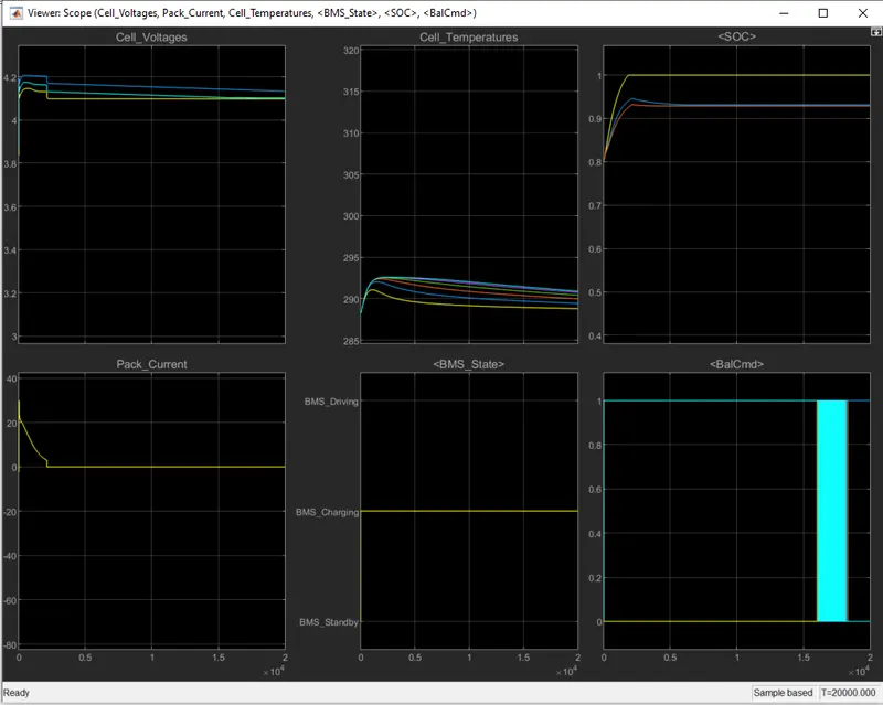
Result

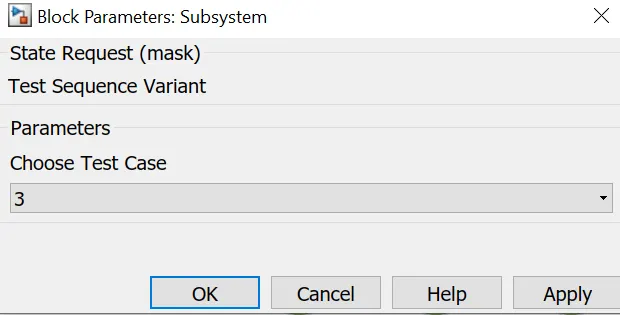
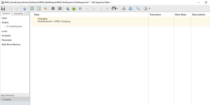
1) The charging condition will be maintained throughout the simulation.

2)There is no driving or standby state in this test.

3) The SOC was set to 80% .

4) After the completion of charging, the pack current increased to 30A and then decreased to O.

5) The voltage of a fully charged cell ranges between 4 and 4.2V.

6) The cell temperatures are also higher at first due to the initial charging current more than 320 level .

2) coulomb counting

The coulomb counting method is also known as the battery current integration method.

In this method. a discharging/charging current is measured and integrated over time to calculate the amount of energy remaining inside the battery. In this method. SOC is taken at the previous step SOC(t-1)and the amount of energy removed/added at the current time step is subtracted/added from the SOC of the previous time step SOC(t-1) to obtain the amount of energy present in the battery at the present instant.

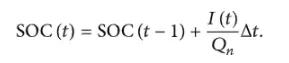
The Coulomb counting method measures the discharging current of a battery and integrates the discharging current over time to estimate SOC. Coulomb counting method is done to estimate the SOC(t). which is estimated from the discharging current. 1(t). and previously estimated SOC values. SOC(t). SOC is calculated by the following equation:

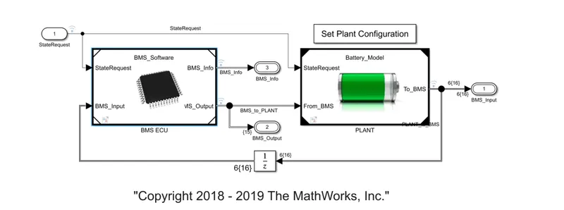
BMS implementation for coulomb counting for SOC estimation

In the BMS ECU subsystem we have

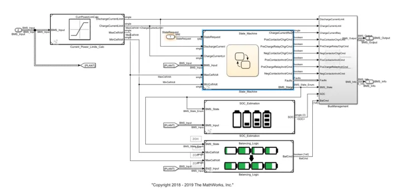
If the SOC estimation block is explored we have

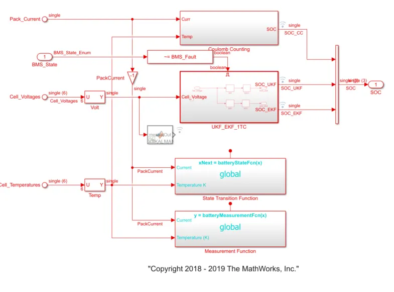
This is the method by which the coulomb counting is implemented.

• Input signals - current and temperature
• Current signal goes to gain block

• Temperature signal goes to the current lookup table.

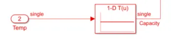
• Both signals are multiplied and divided and output is given to discrete-time integrator to track the safe chargeable time and then SOC is estimated.
• The advantage of this method is its simplicity and low computational cost.