Vehicle Dynamics - ISO Road classification & Road Profile using MATLAB

AIM: Determination of road quality using ISO road classification.

OBJECTIVES: To deliver the following-

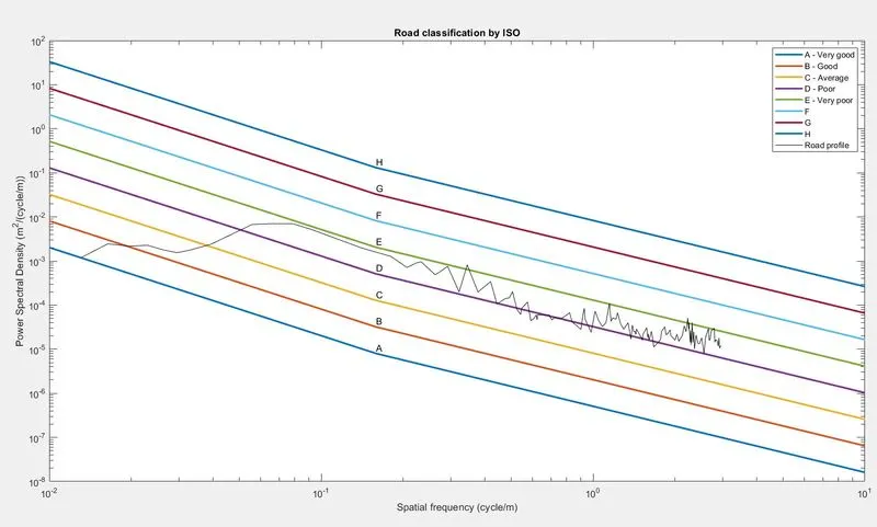
1. Plot showing ISO classification for roads A through H (Use higher end of range for degree of roughness)

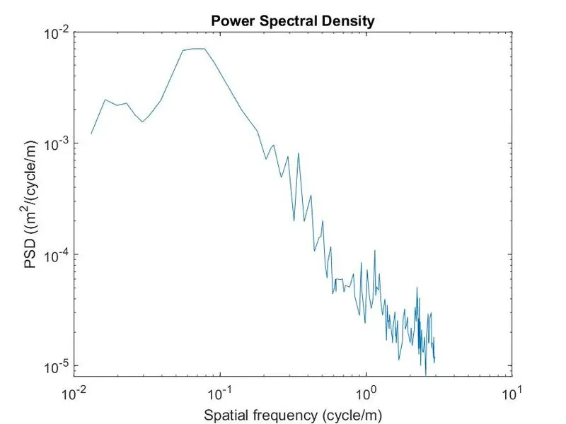
2. Plot showing the PSD profile

3. Overlay of PSD profile on ISO classification and determination of road quality

GIVEN: A data file was given containing the frequencies and corresponding amplitudes of a Road profile test.

( https://drive.google.com/file/d/0B2S2ZJKcURAmeDNFRlMtMm5MSTQ/view )

THEORY:

Road roughness measurement- Road roughness is nothing but the irregularities if the road surface along the longitudinal road travel. The study of road roughness decides the vertical dynamics of the vehicle, i.e., it controls the ride and comfort.

The irregularities as a whole is called as the 'road profile'. In veicle dynamics, we study the road profile using the Spatial frequncy v/s Power Spectral Density (PSD) plots. The PSD is the square of amplitude of the waves that form during the given frequncies. Instead of studying the variation of amplitude we study the power variation wiith respect to the frequency.

ISO road classification- International Organization of Standardization (ISO) has set the road quality criteria by dividing the roads into variouos classes (class A, class B, etc.) depending upon the PSD range which is obtained from the PSD road profile. Note that the PSD is different for for every road. This PSD data is plotted and overlayed with the ISO classification graph; and the combined graph is then studied to determine the road quality.

SOLUTION:

Coding logic-

1. Plotting the PSD from given data:

i) The given PSD data is first immported using the file parsing techniques.

ii) This data is converted to the SI units system and plotted in a seperate figure.

2. Plotting the ISO road classification graphs:

i) All the degrees of roughness values are stored in one two-dimensional array for simplicity.

ii) All the values for S for both the conditions are calculated using a 'for-loop' iterating for the total number of values in degree of roughness variable.

iii) The graph is plotted in another figure window with proper textx, labels and ledgends.

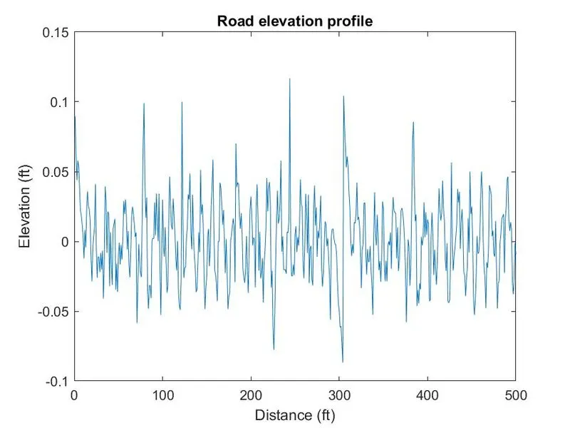
3. Plotting the road elevation profile:

i) The delta sigma for all the given data points is calculated using a for loop exccept for the first and last value. The first and last values are calculated manualy outside the loop because of the formula we are using, there is no value before the first value and no value after the last value, so the code will show an error if we write that in for loop.

ii) The elevation is calculated for all the values for a longitudinal distance of 500ft.

iii) The elevation profile is plotted in a new figure window with prooper labels.

MATLAB code:

clear all
close all
clc

%import given data
data = fopen('PSD_Data.txt');

%getting frequencies 
line1 = fgetl(data);
freq(1) = str2double(line1(9:end));
for i = 2:124
    line = fgetl(data);
    freq(i) = str2double(line);
end
line125 = fgetl(data);
freq(125) = str2double(line125(1:5));

%getting amplitudes
line0 = fgetl(data);
line1 = fgetl(data);
amp(1) = str2double(line1(14:end));
for j = 2:125
    line = fgetl(data);
    amp(j) = str2double(line);
end

%converting the units
freq(:) = freq(:)/0.3048;       %coverting from (cycle/ft) into (cycle/m)
amp(:) = amp(:)*0.3048^3*2*pi;      %converting from (ft^2/(rad/ft)) into (m^2/(cycle/m))

figure(1)
loglog(freq,amp)
title('Power Spectral Density')
xlabel('Spatial frequency (cycle/m)')
ylabel('PSD ((m^2/(cycle/m)')

saveas(1,'psd_given_dataset','jpeg')

%%
%three frequecneis (cycle/m)
omega(1) = 0.01;
omega(2) = 1/(2*pi);
omega(3) = 10;

%road roughness lines
%declaring the degrees of roughness for different road classes
%creating a single array for all the S values
%(A=1,B=2,C=3,D=4,E=5,F=6,G=7,H=8)
s(1,2) = 8e-6;
s(2,2) = 32e-6;
s(3,2) = 128e-6;
s(4,2) = 512e-6;
s(5,2) = 2048e-6;
s(6,2) = 8192e-6;
s(7,2) = 32768e-6;
s(8,2) = 131072e-6;

for m = 1:length(s(:,2))
    s(m,1) = s(m,2)*(omega(1)/omega(2))^-2;
    s(m,3) = s(m,2)*(omega(3)/omega(2))^-1.5;
end

figure(2)
loglog(omega,s,'linewidth',2)
hold on
loglog(freq,amp,'color','black')
title('Road classification by ISO')
xlabel('Spatial frequency (cycle/m)')
ylabel('Power Spectral Density (m^2/(cycle/m))')
text(omega(2),s(1,2),'A','verticalalignment','bottom')
text(omega(2),s(2,2),'B','verticalalignment','bottom')
text(omega(2),s(3,2),'C','verticalalignment','bottom')
text(omega(2),s(4,2),'D','verticalalignment','bottom')
text(omega(2),s(5,2),'E','verticalalignment','bottom')
text(omega(2),s(6,2),'F','verticalalignment','bottom')
text(omega(2),s(7,2),'G','verticalalignment','bottom')
text(omega(2),s(8,2),'H','verticalalignment','bottom')
legend('A - Very good','B - Good','C - Average','D - Poor','E - Very poor','F','G','H','Road profile')

%%
%space domain profile from roughness PSD

delta_sigma(1) = freq(2) - freq(1);
delta_sigma(125) = freq(125) - freq(124);

for k = 2:124
    delta_sigma(k) = (freq(k+1)-freq(k-1))/2;
end

for i = 1:500
    x(i) = i;
    total(i) = 0;
    for j = 1:125
        z(j) = sqrt(amp(j)*2*delta_sigma(j));
        total(i) = total(i) + z(j)*sin(freq(j)*x(i)*2*pi);
    end
end

figure(3)
plot(x,total);
title('Road elevation profile')
xlabel('Distance (ft)')
ylabel('Elevation (ft)')

saveas(3,'road_elevation_profile','jpeg')

PLOTS:

1. PSD Profile

2. ISO road classification

3. Road elevation profile

CONCLUSION: The road profile study using the ISO classification is completed and the required graphs have been plotted successfully using an errorless MATLAB script.