Vehicle Dynamics - Four Wheel Steering

AIM: To study and simulate the 4WS model for steady state.

OBJECTIVES:

1. Derive the `delta_f/delta_r` formula for zero side slip

2. Plot the ratio against forward speed

3. Conclusions from the plot

SOLUTION:

I. Derivation for `delta_f/delta_r` formula for zero side slip:

The state space representation of the 4WS vehicle system is given as:

`d/dt[[v], [r]] = [[-(C_(alpha_f)+C_(alpha_r))/(m*u), (b*C_(alpha_r)-a*C_(alpha_f))/(m*u)-u], [(b*C_(alpha_r)-a*C_(alpha_f))/(I_z*u), -(a^2*C_(alpha_f)+b^2*C_(alpha_r))/(I_z*u)]]*[[v],[r]]+[[C_(alpha_f)/m , C_(alpha_r)/m],[(a*C_(alpha_f))/I_z, -(b*C_(alpha_r))/I_z]]*[[delta_f],[delta_r]]`

where,

`m=>` mass of the vehicle

`I_z=>` yaw moment of inertia

`v =>` lateral speeed

`u =>` longitudinal speed

`r =>` yaw rate

`C_(alpha_f), C_(alpha_r) =>` Front and Rear con=rnering stiffness respectively

`a, b =>` CG distances from front and rear axle respectively

`delta_f, delta_r =>` Front and Rear steering angles respectively

Assuming steady state, i.e.,

`(dv)/dt = 0; (dr)/dt = 0`

`=> [[0], [0]] = [[-(C_(alpha_f)+C_(alpha_r))/(m*u), (b*C_(alpha_r)-a*C_(alpha_f))/(m*u)-u], [(b*C_(alpha_r)-a*C_(alpha_f))/(I_z*u), -(a^2*C_(alpha_f)+b^2*C_(alpha_r))/(I_z*u)]]*[[v],[r]]+[[C_(alpha_f)/m , C_(alpha_r)/m],[(a*C_(alpha_f))/I_z, -(b*C_(alpha_r))/I_z]]*[[delta_f],[delta_r]]`

For zero sideslip angle,

`v = 0, because beta = v/u`

The above equation then becomes

`[[0],[0]] = [[((b*C_(alpha_r)-a*C_(alpha_f))/(m*u)-u)*r],[-((a^2*C_(alpha_f)+b^2*C_(alpha_r))/(I_z*u))*r]]+[[(C_(alpha_f)*delta_f+C_(alpha_r)*delta_r)/m],[(a*C_(alpha_f)*delta_f-b*C_(alpha_r)*delta_r)/(I_z)]]`

after solving this equation, we get

`delta_f = (a*r)/u + (m*b*u*r)/(C_(alpha_f)*L)` and

`delta_r = (m*a*u*r)/(C_(alpha_r)*L) - (b*r)/u`

and the ratio of these two angles,

`delta_f/delta_r = -C_(alpha_r)/C_(alpha_f)*((a*C_(alpha_f)*L + m*b*u^2))/((b*C_(alpha_r)*L - m*a*u^2))`

where,

`L =>` Wheelbase = `a+b`

II. Plotting the ratio against forward speed:

We use a MATLAB script to plot the graph of `delta_f/delta_r` against `u`, i.e., forward speed.

The ratio is plotted for a range of 0 to 50m/s of forward speed.

MATLAB Code:

clear all
close all
clc

%inputs
m = 1000;   %weight of vehicle in kg
Iz = 1400;  %yaw moment of inertia in kgm^2
L = 2.54;   %wheelbase in m
a = 1.14;   %CG distance from front axle in m
Caf = 2400*180/pi;  %front cornering stiffness in N/rad
Car = 2000*280/pi;  %rear cornering stiffness in N/rad
b = L-a;    %CG distance from rear axle in m
r = 0.5;        %yaw rate

%speed range
u = 0:0.1:50;     %speed in m/s


%steering angle ratio
for i = 1:length(u)
    ratio_del(i) = -(Car/Caf)*(a*Caf*L + m*b*u(i)^2)/(b*Car*L - m*a*u(i)^2);        %del_f/del_r
end

%plot
figure(1)
plot(u,ratio_del,'linewidth',2)
xlabel('Longitudinal Speed (m/s)')
ylabel('del_f/del_r')
grid on
saveas(1,'4ws_del_ratio','jpeg')

PLOT:

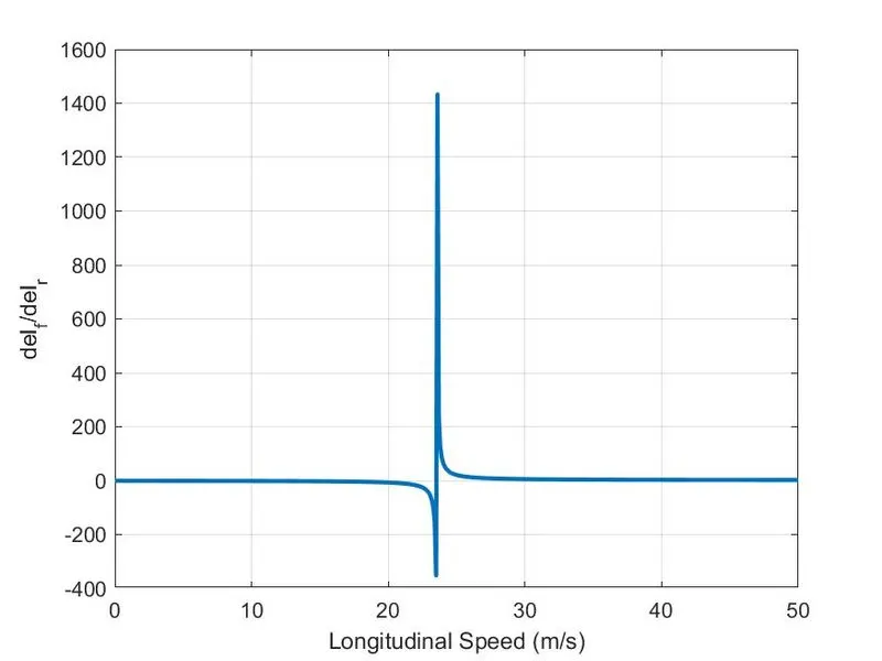
CONCLUSION:

The plot shows that we get a shockwave at 23.5m/s to 23.6m/s. Shockwaves are generally ignored when the vehicle is at high speeds. At low speeds, we need to minimise this wave.