Rankine cycle Simulator using MATLAB

AIM: To write a MATLAB code for simulating a RANKINE CYCLE

OBJECTIVES:

1. Create a code to simulate a Rankine Cycle, the code should calculate the state points based on user inputs.
2. Using the ‘XSteam.m’ function, which is the standard XSteam library for steam table data of water, to determine the required state point variables.
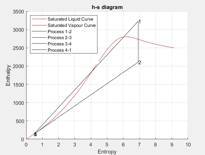
3. Plot the corresponding T-s and h-s diagrams for the given set of inputs.

INTRODUCTION:

Rankine Cycle: The Rankine cycle is the fundamental operating cycle of all power plants where an operating fluid is continuously evaporated and condensed. Rankine cycle is a vapor power cycle which uses a fluid (mainly steam) for all its operation.

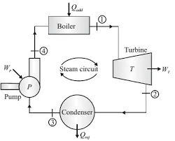
In a Rankine cycle power plant, the boiler heats the water at a very high temperature which converts it into high pressure steam. This steam is used to generate work from the turbine. Further the steam is fed to a condenser which cools it and converts into liquid and this liquid is passed to the pump. The pump requires external work in order to feed this water again to the boiler. All these processes comprise a cycle.

This process is shown in the figure below:

(Image: www.imbooz.com )

Thermodynamically, following are the processes:

1. Process 1-2: The high-pressure steam from the boiler enters in turbine and produces some work, this work is said work done by the turbine. This process is adiabatic expansion meaning the volume increases, this is also called as Isentropic process.
2. Process 2-3: After getting out of the turbine, the steam loses its pressure and is now passed to a condenser which cools it down. Hence, this process is heat rejection process and we call this heat as Q
3. Process 3-4: The cooled steam from the condenser is now a liquid which is passed to the pump. The pump feeds this water at low pressure to the boiler at a high pressure. External work is required to be done on the pump for this purpose. For increasing the pressure, the water is compressed, hence this process is adiabatic compression / isentropic.
4. Process 4-3: in this process the water obtained from pump is heated to a high temperature to convert it into steam which is then used to generate work from turbine. To increase the temperature, the boiler is heated externally. i.e, heat is added into the whole system. This process is isobaric heat addition process, and the heat supplied to the boiler is called Q_in.

Rankine Cycle Simulator:

Simulation in computer programming means creating a mathematical model to predict the behavior or outcome of a real-world practical, physical system. A model built like this is called a simulator.

We are building a Rankine Cycle Simulator using MATLAB programming. This simulator will determine the behavior of the Rankine cycle based on the inputs that would be provided by the user. When the program is run, the results of the Rankine cycle will be obtained in form of data or values of certain thermodynamic entities. The graphs which are the main set of information that determines the performance of the Rankine cycle are also plotted with our simulator.

The program will simply take the inputs from the user and calculate all the data which governs the Rankine cycle.

PROCEDURE:

1. In order to simulate a Rankine cycle, we need some data which in this case is the ‘turbine inlet pressure’, ‘turbine inlet temperature’ and the ‘condenser inlet pressure’. These values should be specified by the user.

Use the ‘input’ command to prompt an appropriate message and take the value typed by the user as the suitable property.

2. You can print the information about the four processes in the command window using the ‘fprintf’ command which is generally used to write data in a text file.
3. There are keywords given in the ‘XSteam’ library which we can use to determine the thermodynamic properties as a function of known quantities.

For this search for the keyword in the ‘XSteam’ file. And use that as argument for the ‘XSteam()’ function.

All the state variables at all the state points can be determined from this and with some thermodynamic relations.

4. Once all the state variables are determined, we can calculate the work and heat involved in the cycle. Net work can be determined and the efficiency is then easily calculated.
5. Now to plot the T-s and h-s diagrams we first draw the saturation line and for that we need a temperature range array containing temperature all values with proper interval in between them. Use ‘linspace’ command to create this array and store the values is a suitable variable.
6. For all these temperature values, determine the specific entropies and enthalpies of saturated liquid and vapour. This is done by using a for-loop which runs from the starting point to the end point of the temperature array. Store the values of these properties in appropriate variables.
7. Plot these saturation points in the T-s graph and the h-s graph with proper respect to each other. Make sure to plot these two in separate figure windows to have both the graphs at the same time.
8. Plot all the state points in both the figures, give proper label to the axes and give a title to both the graphs.
9. All the outputs have been determined at this point. For displaying the results in the command window, use the ‘fprintf’ command and write proper information to be prompted. Write the variables for the corresponding information very carefully.

CODE:

%program to simulate BASIC RANKINE CYCLE

clear all
close all
clc

%take input from user
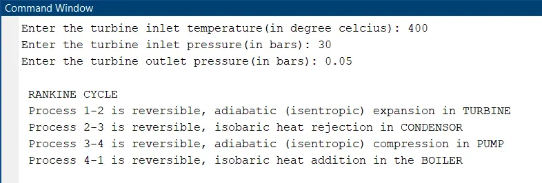
T1 = input('Enter the turbine inlet temperature(in degree celcius): '); 
P1 = input('Enter the turbine inlet pressure(in bars): ');
P2 = input('Enter the turbine outlet pressure(in bars): ');


%display process information
fprintf('n RANKINE CYCLE');
fprintf('n Process 1-2 is reversible, adiabatic (isentropic) expansion in TURBINE');
fprintf('n Process 2-3 is reversible, isobaric heat rejection in CONDENSOR');
fprintf('n Process 3-4 is reversible, adiabatic (isentropic) compression in PUMP');
fprintf('n Process 4-1 is reversible, isobaric heat addition in the BOILER');

%% determinig state variables

%at state point 1
s1 = XSteam('s_pT',P1,T1);
h1 = XSteam('h_pT',P1,T1);

%at staet point 2
s2 = s1;
sf2 = XSteam('sL_p',P2);    %sp. entropy of saturated liquid
sg2 = XSteam('sV_p',P2);    %sp. entropy of saturated vapour
sfg2 = sg2 - sf2;
x = (s2-sf2)/sfg2;         %calculating the dryness fraction
hf2 = XSteam('hL_p',P2);    %sp. enthalpy of saturated liquid
hg2 = XSteam('hV_p',P2);    %sp. enthalpy of saturated vapour
hfg2 = hg2 - hf2;
h2 = hf2 + x*hfg2;

T2 = XSteam('T_hs',h2,s2);  %temperature at point 2,outlet temp from turbine

%work done by the turbine
WT = h1 - h2;

%at state point 3
P3 = P2;        %process 2-3 is isobaric
s3 = sf2;       
h3 = hf2;
V3 = XSteam('vL_p',P3);
T3 = XSteam('T_hs',h3,s3);

%work done on pump
WP = V3*(P1 - P3)*100;      %multiply by 100 to convert into equivalent SI units

%at state point 4
P4 = P1;
h4 = WP + h3;       % WP = h4 - h3
T4 = XSteam('T_ph',P4,h4);
s4 = XSteam('s_pT',P4,T4);

%heat calculations
Qin = h1 - h4;      %heat addition in boiler
Qout = h2 - h3;     %heat rejection in condenser

%net work
Wnet = WT - WP;

%thermal efficiency of rankine cycle
therm_effi = 1 -  (Qout/Qin);

%specific steam consumption
SSC = 3600/Wnet;

%back work ratio
BWR = WP/WT;


%% plotting T-s and h-s diagrams

%setting range for plotting graphs
T = linspace(0,375,1000);

%determining all the required specific enthalpies and entropies for all the
%temperature values in the temperature range
for i = 1:length(T)
    sf(i) = XSteam('sL_T',T(i));
    sg(i) = XSteam('sV_T',T(i));
    hf(i) = XSteam('hL_T',T(i));
    hg(i) = XSteam('hV_T',T(i));
end


%plotting T-s curve
figure(1)
hold on
title('T-s diagram')

%saturation temperature and entropy at boiler process
T5 = XSteam('Tsat_p',P1);
s5 = XSteam('sL_T',T5);     %sp. entropy of saturated liquid 
T6 = T5;                    %saturation temp ffor vapour will be equal throughout in the boiler
s6 = XSteam('sV_T',T6);     %sp. entropy of saturated vapour

%plotting the saturation curve
plot(sf,T,'color','r')
plot(sg,T,'color','r')
xlabel('Entropy')
ylabel('Temperature')
grid on

%plotting processes lines
plot([s1 s2],[T1 T2],'color','black')
plot([s2 s3],[T2 T3],'color','black')
plot([s3 s4],[T3 T4],'color','black')
plot([s4 s5],[T4 T5],'color','black')
plot([s5 s6],[T5 T6],'color','black')
text(s1,T1,'1')
text(s2,T2,'2')
text(s3,T3,'3')
text(s4,T4,'4')

sl = linspace(s6,s1,1000);      

for j = 1:length(sl)
    Tl(j) = XSteam('T_ps',P1,sl(j));
end

plot(sl,Tl,'color','black')


%plotting h-s
figure(2)
hold on
title('h-s diagram')
%plotting the saturation curve
plot(sf,hf,'color','r')
plot(sg,hg,'color','r')
xlabel('Entropy')
ylabel('Enthalpy')
grid on

%plotting processes lines
text(s1,h1,'1')
text(s2,h2,'2')
text(s3,h3,'3')
text(s4,h4,'4')
plot([s1 s2],[h1 h2],'color','black')
plot([s2 s3],[h2 h3],'color','black')
plot([s3 s4],[h3 h4],'color','black')
plot([s4 s1],[h4 h1],'color','black')

legend('Saturated Liquid Curve','Saturated Vapour Curve','Process 1-2','Process 2-3','Process 3-4','Process 4-1','location','northwest')


%% displaying results in command window

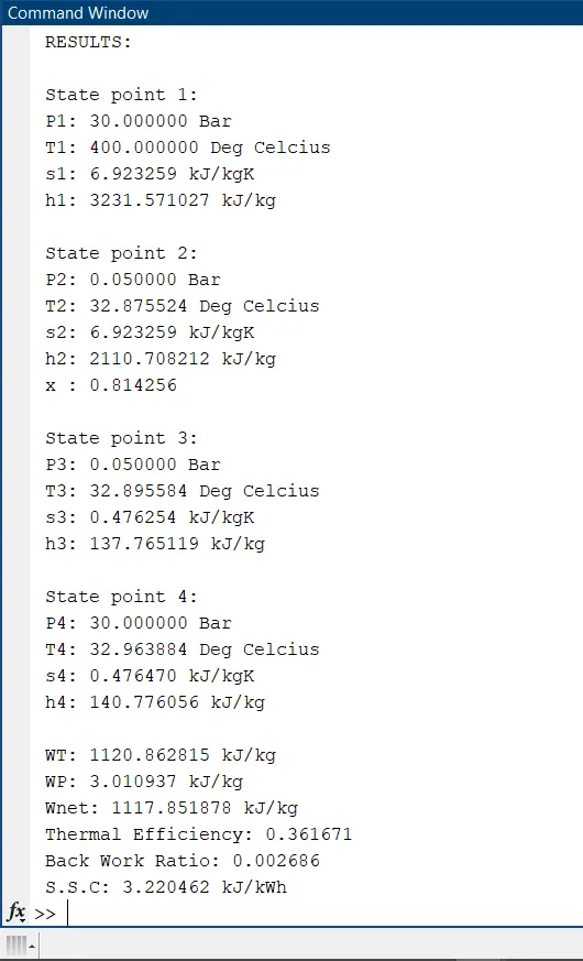
fprintf('nn RESULTS:')

fprintf('nn State point 1:')
fprintf('n P1: %f Bar',P1)
fprintf('n T1: %f Deg Celcius',T1)
fprintf('n s1: %f kJ/kgK',s1)
fprintf('n h1: %f kJ/kg',h1)

fprintf('nn State point 2:')
fprintf('n P2: %f Bar',P2)
fprintf('n T2: %f Deg Celcius',T2)
fprintf('n s2: %f kJ/kgK',s2)
fprintf('n h2: %f kJ/kg',h2)
fprintf('n x : %f',x)

fprintf('nn State point 3:')
fprintf('n P3: %f Bar',P3)
fprintf('n T3: %f Deg Celcius',T3)
fprintf('n s3: %f kJ/kgK',s3)
fprintf('n h3: %f kJ/kg',h3)

fprintf('nn State point 4:')
fprintf('n P4: %f Bar',P4)
fprintf('n T4: %f Deg Celcius',T4)
fprintf('n s4: %f kJ/kgK',s4)
fprintf('n h4: %f kJ/kg',h4)

fprintf('nn WT: %f kJ/kg',WT)
fprintf('n WP: %f kJ/kg',WP)
fprintf('n Wnet: %f kJ/kg',Wnet)
fprintf('n Thermal Efficiency: %f%',therm_effi)
fprintf('n Back Work Ratio: %f',BWR)
fprintf('n S.S.C: %f kJ/kWh',SSC)

fprintf('n')

OUTPUT:

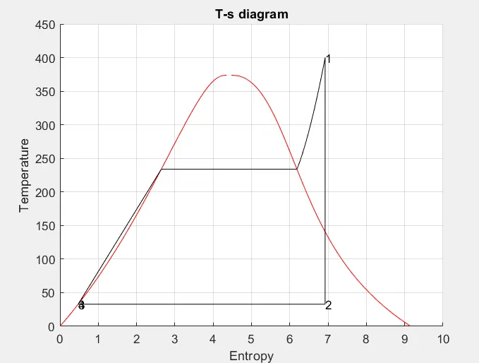
PLOTS:

1. Temperature-Entropy diagram:

2. Enthalpy-Entropy diagram:

CONCLUSION:

The code for simulating a basic Rankine cycle has been written using MATLAB. The program takes inputs from the user and solves the Rankine cycle based on those given inputs.

The T-s and h-s diagrams have been plotted for the Rankine cycle.

In the same we can simulate any thermodynamic cycle using MATLAB programming.

REFERENCES:

1. https://www.sfu.ca/~mbahrami/ENSC%20461/Notes/Vapor%20Power%20Cycles.pdf
2. https://en.wikipedia.org/wiki/Rankine_cycle#:~:text=The%20Rankine%20cycle%20is%20an,heat%20source%20and%20heat%20sink.
3. https://www.ikbooks.com/home/samplechapter?filename=80_Sample_Chapter.pdf
4. https://www.thermopedia.com/content/1072/
5. https://imbooz.com/technical-articles/efficiency-of-rankine-cycle/
6. https://www.learnthermo.com/T1-tutorial/ch09/lesson-B/pg07.php