Solving second order ODEs using MATLAB

AIM: Write a program in MatlabOctave that will simulate the pendulum motion

OBJECTIVE: Simulate the motion between 0-20 sec, for angular displacement=0, angular velocity=3 rad/sec at time t=0s.

GOVERNING EQUATION:
The differential equation for motion of a pendulum is given by:

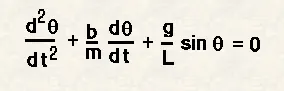
Where, b = damping coefficient

m = mass of the bob (kg)

g = acceleration due to gravity (m/s^2)

L = length of the pendulum (m)

INTRODUCTION: Higher order differential equations are widely used in Engineering field to solve various modern-day problems as well as traditional problems.

Second order differential equations are those whose degree is equal to 2.

In this project we are going to write a MATLAB code to solve an Second Order Differential Equation and create an animation for its motion.

We solve the second order equation by breaking it into two separate first order equation as follows:

1. `(dθ1)/dt = θ2`

2. `(dθ2)/dt = -(b/m)*θ2 - (g/l)*sinθ1`

We write these two equations in form of matrix.

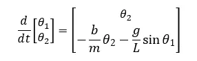
Where, θ₂ = angular displacement

PROCEDURE:

I. For solving ODE and plotting graphs:

1. Declare the values of all the constants in the equation.

b = 0.05, g = 9.81m/s^2, l = 1m, m = 1kg.

2. We write the initial values of angular displacement and angular velocity in a row matrix.
3. Define the time duration for which we want to simulate our equation. Here we simulate for 20 seconds.
4. We solve the given Second ODE using an inbuilt function in MATLAB called ‘ode45’.

‘ode45’ is an ODE solver available in MATLAB. It integrates the given ODE for appropriate limits which we have given in ‘t_span’. ‘ode45’ can solve all the medium order differential equations with great accuracy.

5. We have to define our system of equation in ‘ode45’ for solving that ODE. We created a function that that defines our given equation. We name this function ‘ode_func’.
6. Very carefully provide the inputs in ‘ode45’ in proper order. First, we declare the dependent and independent variables of our equation. Then we call our equation function. Write the timespan and provide the initial conditions.
7. We store the solutions of this in suitable array. We record the time values as well as the displacement and velocity values. The displacement and velocity values are stored in one variable ‘results’.
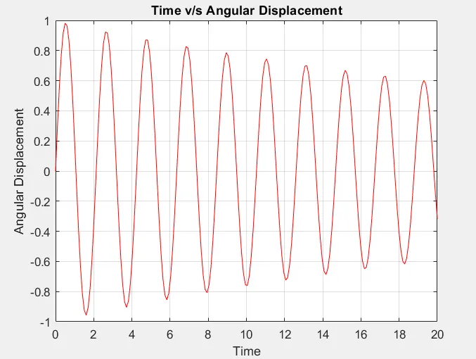
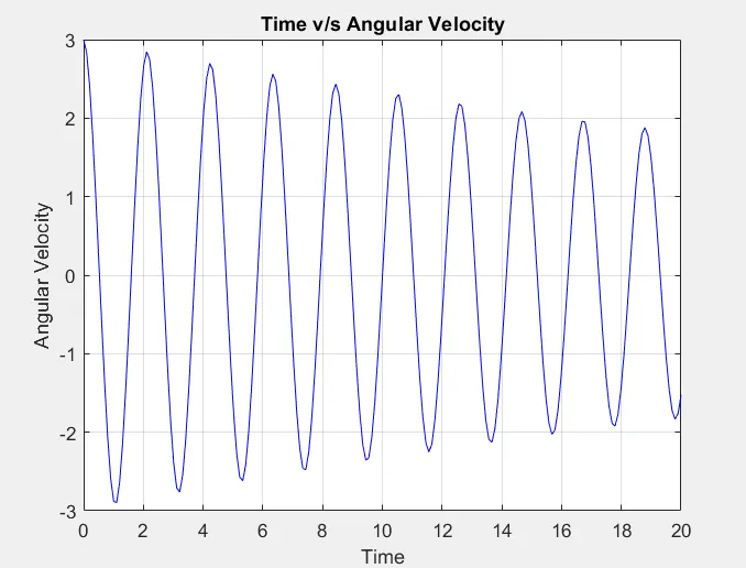
8. We plot the graphs of Angular Displacement & Angular Velocity with respect to time. For this we use values of time ‘t’ and separate values from ‘results.

Give proper title to the graphs and labels to the axes.

II. For creating animation for the motion of pendulum:

1. For creating animation, we use 'for loop' to plot the different positions of the pendulum bob.
2. We run the for loop for the total time period of our motion which is stored in the time ‘t’ variable. So, we iterate the code from 1 to then length of ‘t’.

Length is nothing but the total number of values in ‘t’.

3. Now one end of the pendulum rod/rope is fixed and the other end is freely moving according to our equation. So, the logic is that we draw line between this fixed point and the point which is the current position of the pendulum bob. And with every iteration we will have different position for the bob.
4. We open a figure window and plot the line on the same graph with the help of ‘hold on’ command. Plot a circular marker at the position of free end of the pendulum so that it looks like a pendulum bob. Use ‘markersize’ command to change the size of the marker.
5. When the code is executed the plotting of lines and the marker looks like an animation of pendulum motion.
6. Now for creating a movie of this animation, we use ‘getframe’ command which stores the graphic information of the current figure window in the variable ‘M(c)’.

‘c’ is a counter here; we increase the value of 'c' after every iteration so that we have the information of all the figure windows in a sequence.

7. ‘movie(M)’ command will create a movie of the figure windows. Use ‘VideoWriter’ command to create an AVI file of the movie.
8. When the program is executed we will see the animation in the figure window as the plots are being drawn. Once again MATLAB will play the movie for us.
9. The AVI file of this movie will be created and will be saved in the same folder where our program is saved.

CODE:

close all
clear all
clc

% inputs
b = 0.05;
g = 9.81;
l = 1;
m = 1;

%initial condition
theta_0 = [0; 3];    %initial time = 0sec & initial velocity = 3m/s

%time 
t_span = linspace(0,20,200);    %simulating motion from 0sec to 20seconds

%solving the ode
[t, results] = ode45(@(t, theta) ode_func(t, theta, b, g, l, m), t_span, theta_0);

figure(1)                      
plot(t, results(:,1),'color','r')        %plotting time v/s displacement
ylabel('Angular Displacement')
xlabel('Time')
grid on
title('Time v/s Angular Displacement')

figure(2)
plot(t, results(:,2),'color','b')       %plotting time v/s velocity
ylabel('Angular Velocity')
grid on
title('Time v/s Angular Velocity')
xlabel('Time')


%animation for pendulum motion
c = 1;
for i = 1: length(t)    %running for loop for total time
    theta = results(i,1);
    x0 = 0;               %x-coordinate of fixed position on one end of pendulum
    y0 = 1.5;             %y-coordinate of fixed position on one end of pendulum
    
    x1 = l*sin(theta);    %x-coordinate of other end where bob is attached
    y1 = -l*cos(theta);   %y-coordinate of other end where bob is attached
    
    figure(3)
    
    plot([-1.5 1.5], [1.5 1.5], 'color', 'black', 'linewidth', 2)   %plotting a reference line
    hold on
    axis([-2 2 -2 2])
    grid on
    title('Pendulum Motion')
    plot([x0 x1], [y0 y1], 'color','b')            %plotting line between fixed position and current position of bob
    plot(x1, y1, 'o','markersize',15, 'color','r')   %plotting the bob
    xlabel('Motion in X-direction')
    ylabel('Motion in Y-direction')
    hold off
    M(c) = getframe(gcf);                  %saving current figure window in M(c)
    c = c+1;
    
end

%creating movie of pendulum animation 
movie(M)
videofile = VideoWriter('pendulum_movie.avi', 'uncompressed AVI')
open(videofile)
writeVideo(videofile, M)
close(videofile)

FUNCTION CODE:

function [dtheta_dt] = ode_func(t, theta, b, g, l, m)

theta1 = theta(1);
theta2 = theta(2);

dtheta1_dt = theta2;
dtheta2_dt = -(b/m)*theta2 -(g/l)*sin(theta1);

dtheta_dt = [dtheta1_dt; dtheta2_dt];
end

PLOTS:

1:

2:

CONCLUSION: The motion of pendulum with respect to time has been simulated using MATLAB programming.

We have solved the Second Order Differential Equation by breaking it into two First Order Differential Equations. In the same way, any other differential equation of higher order can be solved using MATLAB.

The movie of animation of the pendulum is created and can be seen from the following link:

https://drive.google.com/drive/folders/1GM5pV27RctbMcobjQST2CPaxmT_qbjel?usp=sharing