Drag Force on a Cyclist using MATLAB

AIM: Write a MATLAB program to calculate drag force against a cyclist.

GOVERNING EQUATION:

Drag Force: Drag Force or Drag is a resisting force experienced by a body moving with some velocity in fluid (ex: Water or Air). The drag force is exerted by the fluid on the body in the opposite direction of motion of the body. Drag Force is also called as the 'Air Resistance'.

Drag Force on a body is calculated by the equation,

`Fd=1/2*rho.A.U^2.Cd`

Where, Fd = drag force (kgm/s^2)

ρ = density of air (kg/m^3)

A = frontal area (m^2)

U = velocity of body (m/s^2)

Cd = drag coefficient

Here, we are studying Flow over Bicycle (with rider). So here the acting fluid is air.

OBJECTIVES: 1. To plot a graph of Velocity v/s Drag force

2. To plot a graph of Drag Coefficient v/s Drag Force

BODY OF THE CONTENT:

I. Plot for Velocity v/s Drag Force

1. Begin the program by writing the following commands to clear all the previous variables and clear the command window:

clear all

close all

clc

2. Create the input variables which are required to calculate the drag force. Assign the values to these variables.

Density of air = 1.225kg/m^3

For Frontal Area , let us consider that the rider is in upright position. In upright position, the frontal area is 0.51m^2

We want to plot the graph between velocity and drag force, hence we need more than one value of both these variables. Therefore, we create an array for values of velocity. let us say that the velocity increases from 0m/s to 20m/s.

3. Create the drag force variable and write the formula. We will get an array containing different values of drag force corresponding to the values of velocity.

4. Use the ‘plot(x, y)’ command to plot the graph between velocity and drag force. We can also give a color to the graph.

5. Label the x and y axes as “Velocity” and “Drag Force” using the ‘xlabel’ and ‘ylabel’ commands respectively. We can enable the grid by using ‘grid on’ command.

Now save the code and run it.

CODE:

clear all
close all
clc

% 1. A plot for Velocity v/s Drag Force

c_d = 1.1;  % cd of air for upright position of rider

A = 0.51;  % Frontal Area in upright position (in meter square)

rho = 1.225;  % Density of  air at STP (in kg/meter cube)

U = linspace(0,20,11)  %Velocity range array (in meter/second squae)

Fd = 0.5*rho*A.*U.^2*c_d  % Drag Force array for different values of U

plot(U, Fd,'color','r')
xlabel('Velocity')
ylabel('Drag Force')
grid on

RESULT:

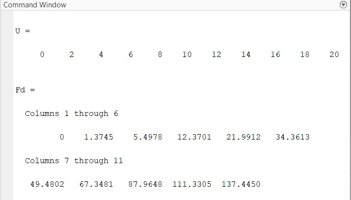
GRAPH:

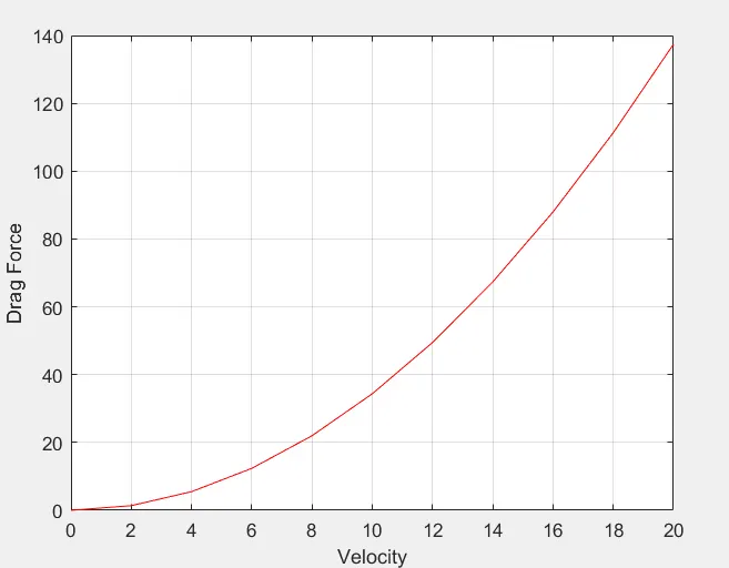
II. Plot for Drag Coefficient v/s Drag Force

1. Begin the program by writing the following commands to clear all the previous variables and clear the command window:

clear all

close all

clc

2. Create the input variables which are required to calculate the drag force. Assign the values to these variables.

Here, we are plotting a graph between drag coefficient and drag force, hence we keep all the other terms constant. And create a range array for coefficient of drag, which varies from 0.6 to 0.8.

Density of air = 1.225kg/m^3

Frontal Area = 0.51m^2 for upright position of rider.

Let us consider that the bicycle moves with a velocity of 30m/s.

3. Create the drag force variable and write the formula. We will get an array containing different values of drag force corresponding to the values of drag coefficient.

4. Use the ‘plot(x, y)’ command to plot the graph between drag coefficient and drag force. We can also give a color to the graph.

5. Label the x and y axes as “Drag Coefficient” and “Drag Force” using the ‘xlabel’ and ‘ylabel’ commands respectively. We can enable the grid by using ‘grid on’ command.

Now save the code and run it.

CODE:

close all
clear all
clc 


% 2. A plot for Drag Coeffecient v/s Drag Force

rho = 1.225;  % Density of air at STP

A = 0.51;  % Frontal Area in upright position of rider

V = 30;  % Constant Velocity 

c_d = 0.6:0.05:0.8  % Drag Coeffecient range array

Fd = 0.5*rho*A*V*V.*c_d  % Drag Force array for different values of c_d

plot(c_d, Fd, 'color', 'b')
xlabel('Drag Coeffecient')
ylabel('Drag Force')
grid on

RESULT:

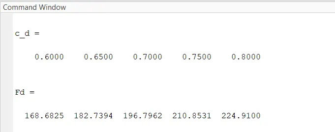
GRAPH:

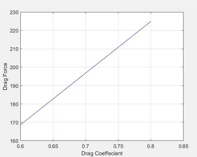
CONCLUSION:

1. From the plot of Velocity v/s Drag Force, we can see that the graph is parabolic. Also from the equation too it is clear that if we double the velocity, the drag force is increased by four times.

2. From the plot of Drag Coefficient v/s Drag Force, we conclude that drag force varies linearly with drag coefficient. There is a direct relation between drag force and drag coefficient. (Note that we have kept all the other terms constant)