Genetic Algorithm in MATLAB to Optimize a given mathematical function

AIM: To understand the concept of Genetic Algorithm and to write a MATLAB code to Optimize the Stalagmite Function.

OBJECTIVES:

1. Write a code in MATLAB to optimise the stalagmite function and find the global maxima of the function.
2. Clearly explain the concept of genetic algorithm in your own words and also explain the syntax for ga in MATLAB in your report.
3. Make sure that your code gives the same output, even if it is made to run several times.
4. Plot graphs for all 3 studies and for F maximum vs no. of iterations. Title and axes labels are a must, legends could be shown if necessary.

INTRODUCTION:

Stalagmite Function: The stalagmite function is defined as follows

`f(x,y) = f1x.f2x.f1y.f2y`

where, `f1x = [sin(5.1pix+0.5)]^6`

`f1y = [sin(5.1piy+0.5)]^6`

`f2x = exp[-4ln(2).(x-0.667)^2/0.64]`

`f2y = exp[-4ln(2).(y-0.667)^2/0.64]`

Defining the function in Matlab Code:

For solving this function for the 'global maxima', we use a negative sign (-) to our main function defination.

We do this because, in matlab, the 'ga' solver determines the 'global minima' of a given function. In order to determine the maxima we inverse the graph of the function so the 'ga' will determine the negative minima which if we take negative will be the same value for 'global maxima' in the positive direction.

function [F] = stalagmite_func(inputs)
x = inputs(1);
y = inputs(2);

f1x = [sin(5.1*pi*x + 0.5)]^6;
f1y = [sin(5.1*pi*y + 0.5)]^6;

f2x = exp(-4*log(2)*((x - 0.0667)^2)/0.64);
f2y = exp(-4*log(2)*((y - 0.0667)^2)/0.64);

F = -f1x*f2x*f1y*f2y;
end 

Genetic Algorithm: Genetic Algorithm is a technique which is derived from biological genetic algorithm and natural selection process. It is used to solve difficult optimization problems and find their corresponding optimum or near-optimum values. This is done by finding the minimum or maximum values of the given function.

This involves taking the best attributes of previous two generations, sometimes mutating the both, sometimes crossing and creating a new offspring of current generation with the best values of the parents.

Five phases are considered in a genetic algorithm.

1. Initial population
2. Fitness function
3. Selection
4. Crossover
5. Mutation

In computational solving, the genetic algorithm for solving a given mathematical function, assumes random input values from the space and evaluates the optimum solution.

Optimization: Optimization is to make the best or most effective of a situation. In any process we have a set of inputs and based n the process we obtain a set of outputs. Now in optimization we find the best possible values of the inputs for which the output will be maximum or minimum.

‘ga’ syntax in matlab:

following is a list of syntaxes we use in the main program to use the 'ga' solver.

x = ga(fun,nvars)

x = ga(fun,nvars,A,b)

x = ga(fun,nvars,A,b,Aeq,beq)

x = ga(fun,nvars,A,b,Aeq,beq,lb,ub)

x = ga(fun,nvars,A,b,Aeq,beq,lb,ub,nonlcon)

x = ga(fun,nvars,A,b,Aeq,beq,lb,ub,nonlcon,options)

x = ga(fun,nvars,A,b,[],[],lb,ub,nonlcon,IntCon)

x = ga(fun,nvars,A,b,[],[],lb,ub,nonlcon,IntCon,options)

note that ‘ga’ only evaluates the minimum value for a given function.

description of each syntax:

1. x= ga(fun,nvars)finds a local unconstrained minimum, x, to the objective function, fun. nvars is the dimension (number of design variables) of fun.

2. x= ga(fun,nvars,A,b)finds a local minimum x to fun, subject to the linear inequalities A*x ≤ b. ga evaluates the matrix product A*x as if x is transposed (A*x').

3. x= ga(fun,nvars,A,b,Aeq,beq)finds a local minimum x to fun, subject to the linear equalities Aeq*x = beq and A*x ≤ b. (Set A=[] and b=[] if no linear inequalities exist.) ga evaluates the matrix product Aeq*x as if x is transposed (Aeq*x').

4. x= ga(fun,nvars,A,b,Aeq,beq,lb,ub)defines a set of lower and upper bounds on the design variables, x, so that a solution is found in the range lb ≤ x ≤ ub. (Set Aeq=[] and beq=[] if no linear equalities exist.)

5. x= ga(fun,nvars,A,b,Aeq,beq,lb,ub,nonlcon)subjects the minimization to the constraints defined in nonlcon. The function nonlcon accepts x and returns vectors C and Ceq, representing the nonlinear inequalities and equalities respectively. ga minimizes the fun such that C(x) ≤ 0 and Ceq(x) = 0. (Set lb=[] and ub=[] if no bounds exist.)

6. x= ga(fun,nvars,A,b,Aeq,beq,lb,ub,nonlcon,options)minimizes with the default optimization parameters replaced by values in options. (Set nonlcon=[] if no nonlinear constraints exist.) Create options using optimoptions.

7. x= ga(fun,nvars,A,b,[],[],lb,ub,nonlcon,IntCon)or x = ga(fun,nvars,A,b,[],[],lb,ub,nonlcon,IntCon,options) requires that the variables listed in IntCon take integer values.

PROCEDURE:

1. First, we define our search space bye creating arrays of x values and y values.

Create 2d array for this space range with the help of ‘meshgrid()’ command.

2. Evaluate the function values for this space range using for loop. Run the for from 1 to the length of x values of the 2d array. Now for each x value we want to determine the function value at all the y values.

For this, use another for loop inside the first for loop. Store the values of function in an array.

3. Now we determine the optimum solution for different study cases which are discussed in detail below.
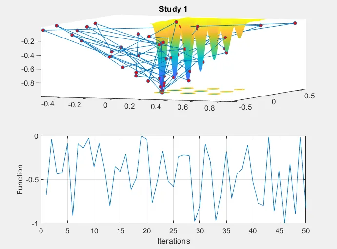
4. In first study, we have not set the limits for ‘ga’ which takes random values from space, i.e., here ‘ga’ will take inputs from all over the space irrespective of our defined spacer range.
5. We solve the solution multiple times using for loop. ‘num_cases’ is the variable which stores the value of number of iterations. Here we set it to 50.
6. Open a figure window and divide it into two parts using the ’subplot()’ command. In the first part plot the surface graph of the given stalagmite function using the values that we have determined. Enable ‘shading interp’ to obtain a smooth colour shaded surface. Also plot the points of optimum solutions from each iteration in the same graph. Give proper labels.
7. Plot the optimum values of the function with respect to the iterations to have a clear visualization of values in the space.
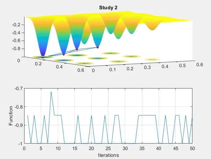
8. In second study, we set the upper and lower limits for ‘ga’ to take values only from that range. Now use the same process as used in study one for determining the function optimum values.
9. Open another figure window and do the same process to plot the surface and optimum points. Also plot the optimum values with respect to the number of iterations.
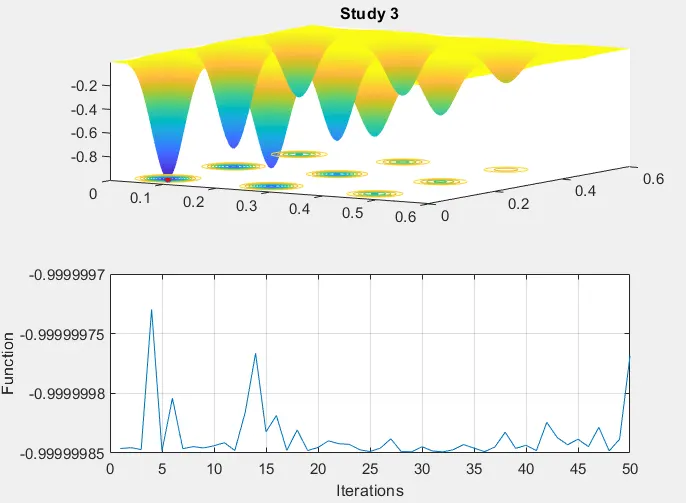
10. In third study, we increase the population size which is the set of individual points that ‘ga’ will take as inputs, i.e, it is the number of optimizations points that ‘ga’ will use while solving the function for each iteration.
11. This will require additional information to be defined in the syntax of ‘ga’. The ‘PopulationSize’ for ‘ga’ is available in the options which are set at default. For using another value for any of these options, ‘optimoptions()’ command is used where by specifying the name of the option we can set a new value for that option.
12. Here we set the ‘PopulationSize’ to 200.
13. For determining the optimum values use for loop to iterate the ‘ga’ multiple times. For each iteration store the values in an array.
14. Open a new figure window and divide it into two parts using the ‘subplot()’ command. In the first part plot the surface of our function and the optimum points obtained from the ‘ga’ solver.
15. In the second part, plot the optimum points with respect to the number of iterations.
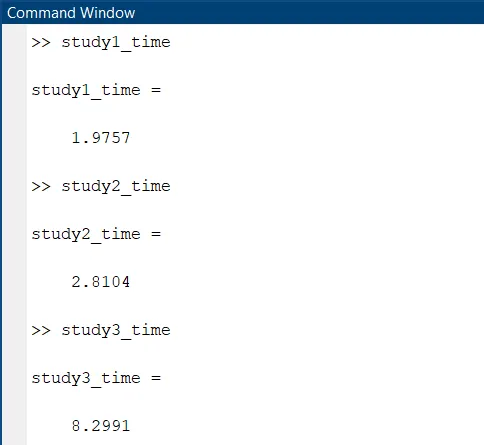
16. For each study we record the time elapsed while solving the funtion. This is done by using the 'tic' & 'toc' in matlab.

CODE:

clear all
close all
clc

%search spcae
x = linspace(0,0.6,150);
y = linspace(0,0.6,150);
num_cases = 50;

%create 2D arrays
[xx, yy] = meshgrid(x, y);

%evaluation of stalagmite
for i = 1:length(xx);
    for j = 1:length(yy);
        inputs(1) = xx(i,j);
        inputs(2) = yy(i,j);
        F(i,j) = stalagmite_func(inputs);
    end
end

%study 1 - without upper and lower bounds
tic
for i = 1:num_cases
    [inputs, Fopt(i)] = ga(@stalagmite_func, 2);
    xopt(i) = inputs(1);
    yopt(i) = inputs(2);
end
study1_time = toc

figure(1)
subplot(2,1,1)
hold on 
surfc(x,y,F)
title('Study 1')
shading interp
plot3(xopt,yopt,Fopt,'marker','o','markersize',4,'markerfacecolor','r')
subplot(2,1,2)
plot(Fopt)
xlabel('Iterations')
ylabel('Function')
grid on

%study 2 - setting upper and lower bounds
tic
for i = 1:num_cases
    [inputs, Fopt(i)] = ga(@stalagmite_func,2,[],[],[],[],[0;0],[0.6;0.6]);
    xopt(i) = inputs(1);
    yopt(i) = inputs(2);
end

study2_time = toc

figure(2)
subplot(2,1,1)
hold on
surfc(x,y,F)
title('Study 2')
shading interp
plot3(xopt,yopt,Fopt,'marker','o','markersize',4,'markerfacecolor','r')
subplot(2,1,2)
plot(Fopt)
xlabel('Iterations')
ylabel('Function')
grid on

%study 3 - increasing the population size of ga
tic
options = optimoptions('ga');
options = optimoptions(options,'PopulationSize',200);
for i = 1:num_cases
    [inputs, Fopt(i)] = ga(@stalagmite_func,2,[],[],[],[],[0;0],[0.6;0.6],[],[],options);
    xopt(i) = inputs(1);
    yopt(i) = inputs(2);
end

study3_time = toc

figure(3)
subplot(2,1,1)
hold on
surfc(x,y,F)
shading interp
title('Study 3')
plot3(xopt,yopt,Fopt,'marker','o','markersize',4,'markerfacecolor','r')
subplot(2,1,2)
plot(Fopt)
xlabel('Iterations')
ylabel('Function')
grid on

Time (in seconds) taken to solve each study case:

PLOTS:

1. Study 1 - Without setting the upper and lower bounds

2. Study 2 - Setting the upper and lower bounds

3. Study 3 - Increasing the population size for ga

CONCLUSION:

1. From the figure of study 1, we can see that the solution is not effective beecause there are input values which are not even in our search space taken by the solver to solve the function. For every iteration there is a major difference between the values of our optimum solution.

2. When we set the upper and lower bounds for 'ga' to take input values from our search space only, it is seen from the graph that now the values are much closer to each other than before. The solution now converges to one global minima and three local minimas. The optimum solution values range from -1 to -0.7. which on a larger scale is a small difference. But the solution is still not effective for micro applications.

3. The initial population is increased to 200 in thhe third study and also the upper and lower bounds are set. Doing this drastically changes the accuracy of the optimum solution. The solution now converges to only one global minima, and the values of solutions for each iterations ranges from -0.99999985 to -0.99999997 which is a much much smaller difference that if we round up to three decimal points the solution remains constant and the value will be approximately -1.

Now as we have taken negative of the function, we have determined the optimum minima or the global minima using the 'ga' solver. If we take the original function, the same value will be of the global maxima with negative sign removed.

Hence, the global maxima of stalagmite function, for the range of x = 0 to 0.6 & y = 0 to 0.6, is found out to be approximately '1'.

REFERENCES:
1. https://www.tutorialspoint.com/genetic_algorithms/genetic_algorithms_introduction.htm

2. https://in.mathworks.com/help/gads/what-is-the-genetic-algorithm.html
3. https://in.mathworks.com/help/gads/ga.html
4. https://in.mathworks.com/matlabcentral/answers/52240-how-to-find-max-fuction-with-genetic-algorithm
5. https://towardsdatascience.com/introduction-to-genetic-algorithms-including-example-code-e396e98d8bf3