Vehicle Dynamics - Transient Handling

AIM: To solve given conceptual numerical question based on 'Transient Handling':

Question- The following table contains information about two vehicles

OBJECTIVES:

1. Calculate the following parameters for both using formulas

1. Undamped natural frequency (Hz)

2. Damping ratio

3. Damped frequency (Hz)

4. Rise time

2. Plot the unit step response of the system for lateral speed, lateral acceleration and yaw rate

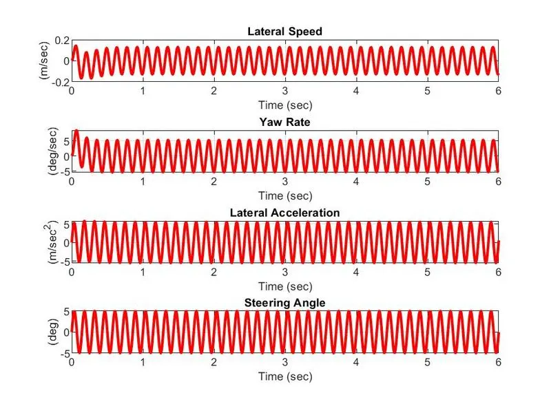
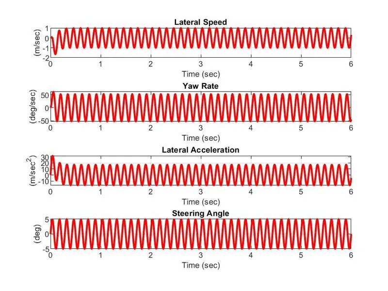
3. Plot the sine response of for lateral speed, lateral acceleration and yaw rate (5 deg, 7hz sine input)

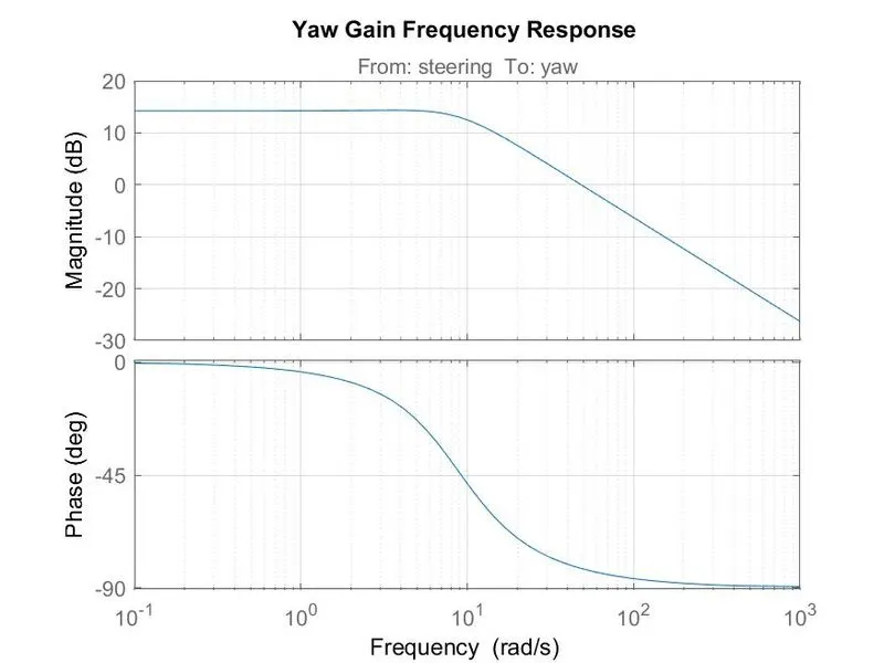
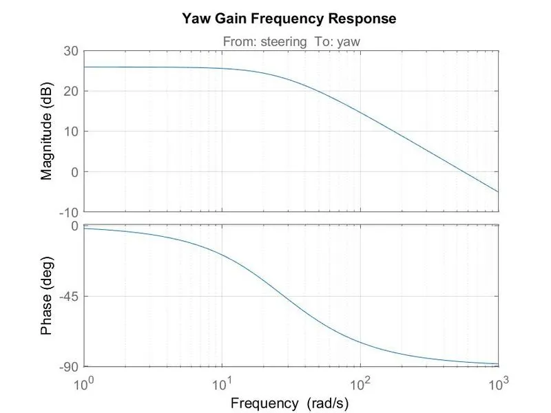
4. Plot the yaw gain (yaw/steering input) in the frequency domain

5. Show correlation for the following (in other words, you should get the same answer between two different methods of calculation)

1. Steady state yaw gain - between the sine response and the frequency response plot

2. Yaw gain at 7hz - between the sine reponse and the frequency response plot

3. Response time - between the step response plot and your analytical calculations

GIVEN: (Suffixes: P- for Passenger car; R- for Race car.)

FWD passenger car-

`W_(Total_P) = 2000lb = 907.184kg`

`W_(f_P) = 65/100*907.184 =589.67kg`

`W_(r_P) = 317.514kg`

`I_(zz_P) = 1128kgm^2`

`L_P = 8.33ft = 2.539m`

`a_P = 2.92ft = 0.89m`

`b_P = 5.41ft = 1.649m`

`C_(alpha_(f_P)) = 13752lb//rad = 61172N//rad`

`C_(alpha_(r_P)) = 11460lb//rad = 50976N//rad`

Formula 1 race car-

`W_(Total_R) = 1719lb = 779.7246kg`

`W_(f_R) = 40/100*1719 = 687.6lb = 311.8899kg`

`W_(r_R) = 1719-687.6 = 1031.4lb = 467.8348`

`I_(zz_R) = 865kgm^2`

`L_R = 9.52ft = 2.9017m`

`a_R = 5.71ft = 1.7404m`

`b_R = 3.81ft = 1.1613m`

`C_(alpha_(f_R)) = 62228lb//rad = 276800N//rad`

`C_(alpha_(r_R)) = 96608lb//rad = 429730N//rad`

SOLUTION:

we know the characteristic equation-

`(MuI_(zz))s^2-(MuN_r + Y_betaI_(zz))s + (Y_betaN_r + N_betaMu - Y_rN_beta) = 0`

and the standard equation-

`s^2 + 2zetaomega_ns + omega_n^2=0`

Therefore,

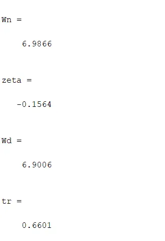
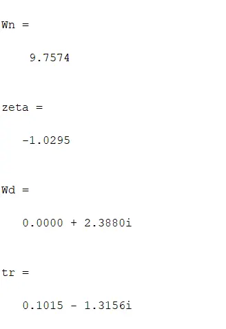
1. The undamped natural frequency:

`omega_n = sqrt((Y_betaN_r+N_betaMu-Y_rN_beta)/(MuI_(zz)))`

where,

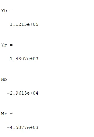
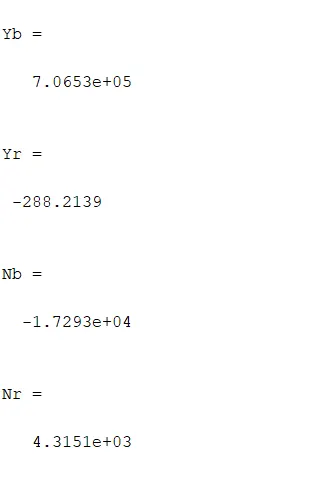
`Y_beta = C_(alpha_f) + C_(alpha_r)`

`Y_r = (aC_(alpha_f) - bC_(alpha_r))/u`

`N_beta = aC_(alpha_f) - bC_(alpha_r)`

`N_r = (a^2C_(alpha_f) - b^2C_(alpha_r))/u`

2. Damping ratio:

`zeta = -(MuN_r + Y_betaI_(zz))/(2omega_n(MuI_(zz)))`

3. Damped frequency:

`omega_d = omega_nsqrt(1-zeta^2)`

4. Rise time:

`t_r = (pi-theta)/omega_d`

where, `theta = arctan((sqrt(1-zeta^2))/zeta)`

I. For FWD Passenger car- (at 20m/sec)

II. For Formula 1 race car- (at 60m/sec)

MATLAB CODE:

%% FWD Passenger Car 
clear all
close all
clc

%inputs
M = 2000*0.453592;      %total weight of car in (kg)
mf = 65*M/100;     %front weight
mr = M - mf;       %rear weight
Izz = 1128;        %yaw moment of inertia in (kg-m^2)
L = 8.33*0.3048;       %wheelbase in (m)
a = 2.92*0.3048;       %CG distance from front axle in (m)
b = L-a;        %CG distance from rear axle in (m)
Cf = 13752*4.4482;        %front cornering stiffness in (N/rad)
Cr = 11460*4.4482;        %rear cornering stiffness in (N/rad)

%speed
u = 20;      %speed in (m/sec)

temp = 0;
%% Formula 1 Race Car
clear all
close all
clc

%inputs
M = 1719*0.453592;      %total weight of car in (kg)
mf = 40*M/100;     %front weight
mr = M - mf;       %rear weight
Izz = 865;        %yaw moment of inertia in (kg-m^2)
L = 9.52*0.3048;       %wheelbase in (m)
a = 5.71*0.3048;       %CG distance from front axle in (m)
b = L-a;        %CG distance from rear axle in (m)
Cf = 62228*4.4482;        %front cornering stiffness in (N/rad)
Cr = 96608*4.4482;        %rear cornering stiffness in (N/rad)

%speed
u = 60;      %speed in (m/sec)

temp = 1;

%% numerical
Yb = Cf+Cr
Yr =(a*Cf-b*Cr)/u
Nb = a*Cf-b*Cr
Nr = (a^2*Cf-b^2*Cr)/u
Yr1 = abs((a*Cf-b*Cr)/u);
Nb1 = abs(a*Cf-b*Cr);
Nr1 = abs((a^2*Cf-b^2*Cr)/u);

Wn = sqrt((Yb*Nr1 + Nb1*M*u - Yr1*Nb1)/(M*u*Izz))
zeta = -(M*u*Nr + Yb*Izz)/(2*Wn*M*u*Izz)
Wd = Wn*sqrt(1-zeta^2)

theta = atan(sqrt(1-zeta^2)/zeta);
tr = (pi - theta)/Wd

%% Simulation
%state space matrices
A = [-(Cf+Cr)/(M*u), (b*Cr-a*Cf)/(M*u) - u
    (b*Cr-a*Cf)/(Izz*u), -(a^2*Cf+b^2*Cr)/(Izz*u)];

B = [Cf/M; a*Cf/Izz];

C_lat = [1, 0]; D_lat = 0;       %lateral speed
C_yaw = [0, 1]; D_yaw = 0;      %yaw rare
C_acc = A(1,:) + u*[0,1]; D_acc = B(1);     %lateral acceleration

C = [C_lat; C_yaw; C_acc];
D = [D_lat; D_yaw; D_acc];

t = 0:0.01:6;
U = (5*pi/180)*sin(7*2*pi*t);       %sine response of 5 deg steering input at 7Hz 

sys = ss(A,B,C,D);      %state space representation

Y = lsim(sys,U,t);      %sinusoidal input

sys.inputname = {'steering'};
sys.outputname = {'lat'; 'yaw'; 'acc'};

%plots

figure(1)
%[mag, w] = bodemag(sys({'yaw'}, 'steering'));
bodeplot(sys({'yaw'}, 'steering'))
grid on
title('Yaw Gain Frequency Response')


figure(2) %step response
step(sys);
grid on


figure(3)   %sine response
%Lateral speed
subplot(4,1,1)
plot(t, Y(:,1),'r','linewidth',2)
grid on
title('Lateral Speed')
xlabel('Time (sec)')
ylabel('(m/sec)')

%yaw rate
subplot(4,1,2)
plot(t, Y(:,2)*180/pi,'r','linewidth',2)
grid on
title('Yaw Rate')
xlabel('Time (sec)')
ylabel('(deg/sec)')

%lateral acceleration
subplot(4,1,3)
plot(t,Y(:,3),'r','linewidth',2)
grid on
title('Lateral Acceleration')
xlabel('Time (sec)')
ylabel('(m/sec^2)')

%steering input
subplot(4,1,4)
plot(t,U*180/pi,'r','linewidth',2)
grid on
title('Steering Angle')
xlabel('Time (sec)')
ylabel('(deg)')


if temp == 0
    saveas(1, 'yawgain_freq_resp_passenger', 'jpeg')
    saveas(2, 'step_resp_passenger', 'jpeg')
    saveas(3, 'sine_resp_passenger', 'jpeg')
else
    saveas(1, 'yawgain_freq_resp_f1', 'jpeg')
    saveas(2, 'step_resp_f1', 'jpeg')
    saveas(3, 'sine_resp_f1', 'jpeg')
end

Coding logic-

We create a system for Transient Handling of a four wheel car using the 2DOF mathmatical model. The system of matirx is created in matlab using the 'ss' function which delivers a state space form of the matrices that are fed into it as arguments.

Here, A and B are the input matrices of a steady state transient handling model. C matrix consist the three main outputs that we need, i.e., lateral speed, yaw rate and lateral acceleration.

There is a matlab function called 'step' which directly plots the step response of the system.

For sine response, we first create a sine input of 5 deg amplitude and 7Hz frequency. This sine input is then used against the parameters to plot the sine response.

The yaw gain frequency response is plotted using the inbuilt 'bodeplot' function which generates a graph of the yaw gain in the frequency domain. Bodeplot is a combination of two plots- magnitude plot, phase plot.

OUTPUTS:

I. For FWD Passenger car- (at 20m/sec)

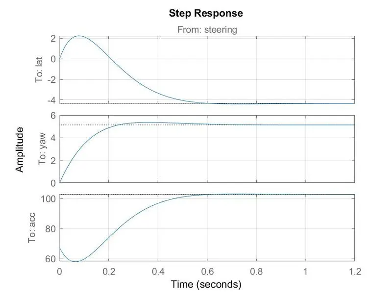
1. Unit Step Response:

2. Sine Response:

3. Yaw Gain Frequency Response:

II. For Formula 1 race car- (at 60m/sec)

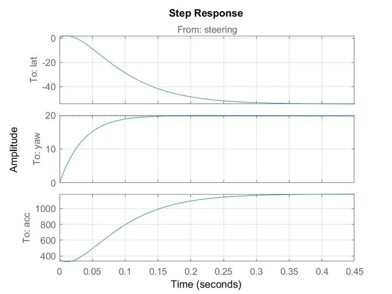
1. Unit Step Response:

2. Sine Response:

3. Yaw Gain Frequency Response:

Inference from the plots-

From the step reponse plots of both the cars, it is observed that the lateral speed goes down and has negative values. The reason behind is that the velocity, as we know, is a vector quantity; the negative values are just indicating that the direction is opposite.

The response time for passenger car is 1.2 seconds and that of the formula 1 car is 0.45 seconds. This means the Formula 1 car responds faster than the Passenger car.

The yaw gain magnitude in the frewuency domain of Formula 1 car is greater than the Passenger car.

CONCLUSION:

We have studied the concept of transient handling and the required graphs were plotted using the model with the help of an errorless MATLAB script.