Vehicle Dynamics - Study on Longitudinal and Lateral force using Pacejka Magic Formula in MATLAB

AIM: To study-

1. The effect of different slip angles on force(Fx and Fy) v/s slip ratio relationship

2. The effect of different slip rations on force(Fx and Fy) v/s slip angle relationship

OBJECTIVES: Deliver the following-

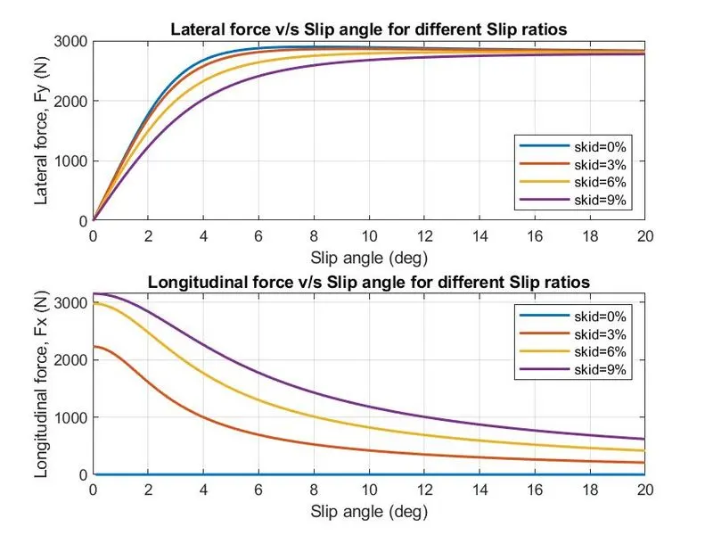
1. Plot (use sub-plots) showing the effect of different slip ratios on lateral force vs slip angle relationship

2. Plot showing the effect of different slip ratios on longitudinal force vs slip angle relationship

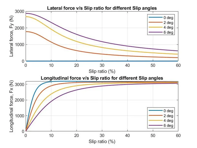
3. Plot showing the effect of different slip angles on longitudinal force vs slip ratio relationship

4. Plot showing the effect of different slip angles on lateral force vs slip ratio relationship

GIVEN:

SOLUTION:

MATLAB Code:

%% for different slip ratios

clear all
close all
clc

%inputs
Sx_p = 0.09;        %peak slip ratio
alpha_p = 4;        %peak slip angle

%pacejka coefficients (given)
By = 0.27; Cy = 1.2; Dy = 2900; Ey = -1.6; Shy = 0; Svy = 0;
Bx = 25; Cx = 1.15; Dx = 3200; Ex = -0.4; Shx = 0; Svx = 0;

save('given_pacejka_coeff')     %saving variables for future use

%iterating for values of slip ratios
for i = 1:4         %slip ratios (0%, 3%, 6%, 9%)
    Sx = (i-1)*0.03;
    
    for j = 1:201
        slip_angle(j) = (j-1)*0.1;
        alpha = slip_angle(j);
        
        %normalized slip factors
        Sx_star = Sx/Sx_p;
        alpha_star = alpha/alpha_p;
        
        %resultant slip
        S_star = ((Sx_star)^2 + (alpha_star)^2)^0.5;
        
        %modified slip factors
        Sx_mod = S_star*Sx_p;
        alpha_mod = S_star*alpha_p;
        
        %LATERAL FORCE
        Alpha = alpha_mod + Shy;
        fy(i,j) = (alpha_star/S_star)*Dy*sin(Cy*atan(By*Alpha-Ey*(By*Alpha-atan(By*Alpha))));
        Fy(i,j) = fy(i,j) + Svy;
        
        %LONGITUDINAL FORCE
        Sxf = Sx_mod + Shx;
        fx(i,j) = (Sx_star/S_star)*Dx*sin(Cx*atan(Bx*Sxf-Ex*(Bx*Sxf-atan(Bx*Sxf))));
        Fx(i,j) = fx(i,j) + Svx;
        
    end
end

figure(1)
subplot(2,1,1)
plot(slip_angle, Fy,'linewidth',1.5)
title('Lateral force v/s Slip angle for different Slip ratios')
xlabel('Slip angle (deg)')
ylabel('Lateral force, Fy (N)')
legend('skid=0%','skid=3%','skid=6%','skid=9%','location','southeast')
grid on

subplot(2,1,2)
plot(slip_angle, Fx,'linewidth',1.5)
title('Longitudinal force v/s Slip angle for different Slip ratios')
xlabel('Slip angle (deg)')
ylabel('Longitudinal force, Fx (N)')
legend('skid=0%','skid=3%','skid=6%','skid=9%')
grid on

saveas(1,'slip_ratio_Fx_Fy','jpeg')

%% for different slip angles
clear all
clc

load('given_pacejka_coeff.mat')     %loading previously saved pacejka coefficients ang given inputs

%iterating for values of slip angle
for i = 1:4     
    slip_angle(i) = (i-1)*2;        %slip angle (0,2,4,6) degrees
    alpha = slip_angle(i);
    
    for j = 1:300
        Sx(j) = (j-1)*0.002;
        
        %normalized slip factors
        Sx_star = Sx(j)/Sx_p;
        alpha_star = alpha/alpha_p;
        
        %resultant slip
        S_star = ((Sx_star)^2 + (alpha_star)^2)^0.5;
        
        %modified slip factors
        Sx_mod = S_star*Sx_p;
        alpha_mod = S_star*alpha_p;
        
        
        %LATERAL FORCE
        Alpha = alpha_mod + Shy;
        fy(i,j) = (alpha_star/S_star)*Dy*sin(Cy*atan(By*Alpha-Ey*(By*Alpha-atan(By*Alpha))));
        Fy(i,j) = fy(i,j) + Svy;
        
        %LONGITUDINAL FORCE
        Sxf = Sx_mod + Shx;
        fx(i,j) = (Sx_star/S_star)*Dx*sin(Cx*atan(Bx*Sxf-Ex*(Bx*Sxf-atan(Bx*Sxf))));
        Fx(i,j) = fx(i,j) + Svx;
        
    end
end

figure(2)
subplot(2,1,1)
plot(Sx*100, Fy,'linewidth',1.5)
title('Lateral force v/s Slip ratio for different Slip angles')
xlabel('Slip ratio (%)')
ylabel('Lateral force, Fy (N)')
legend('0 deg','2 deg','4 deg','6 deg')
grid on

subplot(2,1,2)
plot(Sx*100, Fx,'linewidth',1.5)
title('Longitudinal force v/s Slip ratio for different Slip angles')
xlabel('Slip ratio (%)')
ylabel('Longitudinal force, Fx (N)')
legend('0 deg','2 deg','4 deg','6 deg','location','southeast')
grid on

saveas(2,'slip_angle_Fx_Fy','jpeg')

OUTPUT:

1. Effect of different slip ratios:

2. Effect of different slip angles:

Inference from the plots:

1. Effect of different slip ratios on-

i) Lateral force v/s Slip angle

- There is no lateral force at zero slip angle for all values of skid ratio.

- Lateral force increases with increase in slip angle.

- Maximum lateral force is achieved at 0% skid. And it decreases with increase in skid ratio.

ii) Longitudinal force v/s Slip angle

- Longitudinal force increases with increase in slip angle.

- There is no longitudinal force at 0% skid for all values of slip angle.

- The peak value of longitudinal force is at 0 degree slip angle for all skid ratios. And it is maximum for 9% skid.

2. Effect of different slip angles on-

i) Lateral force v/s slip ratio

- There is no lateral force at zero slip angle.

- Peak value of lateral force for all slip angles occurs at zero% slip ratio.

ii) Longitudinal force v/s slip ratio

- The longitudinal force is zero at 0% slip for all slip angles.

- Longitudinal force is maximum for 0 deg slip angle and decreases with increase in slip angle.

CONCLUSION: The effect of slip angle and slip ratio on Force relationship with slip ratio and slip angle respectively have been plotted using an errorless MATLAB script.