Solving an Air Standard Cycle using MATLAB

AIM: Write a code that can solve an otto cycle and make plots for it.

OBJECTIVES: 1. Create a PV diagram.

2. Output the ‘thermal efficiency’ of the engine.

THEORY:

Otto cycle: Otto cycle is a thermodynamic cycle most commonly found in automobile engines. The cycle describes the functioning of a typical ‘Spark Ignition Piston Engines’.

The Otto cycle is comprised of following processes:

1. Process 1–2 is an adiabatic (isentropic) compression of the charge as the piston moves from bottom dead centre(BDC) to top dead centre (TDC).
2. Process 2–3 is a constant-volume heat transfer to the working gas from an external source while the piston is at top dead centre. This process is intended to represent the ignition of the fuel-air mixture and the subsequent rapid burning.
3. Process 3–4 is an adiabatic (isentropic) expansion (power stroke).
4. Process 4–1 completes the cycle by a constant-volume process in which heat is rejected from the air while the piston is at bottom dead centre.

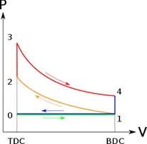(image: Wikipedia)

GOVERNING EQUATIONS:

1. For process 1-2:

P1.V1^γ = P2.V2^γ

P1.V1/T1 = P2.V2/T2

2. For process 2-3:

P2.T2 = P3.T3

3. For process 3-4:

P3.V3^γ = P4.V4^γ

Where, P = pressure at corresponding points

V = volume at corresponding points

T = temperature at corresponding points

γ = specific heat ration = Cp/Cv

4. Volume Trace of engine cylinder:

Where, V = volume trace

Vc = clearance volume

Cr = compression ratio

R = ratio of connecting rod length to crank pin radius

Θ = crank angle

5. Thermal Efficiency:

Efficiency = 1 + (T1 - T4)/(T3 - T2)

PROCEDURE:

1. We start by declaring the variables for state point 1. The volume at first and second point will be the volumes of the engine cylinder when the piston is moving.
2. The volume at point 1 will be equal to the total volume of the empty cylinder, which is the swept volume plus clearance volume. And that at the point 2 will be equal to the clearance volume when the piston is at TDC.
3. The pressure at point 2 can be calculated from the appropriate equation.
4. Similarly, all the other state variables for all the state points can be determined and should be declared in the code carefully.
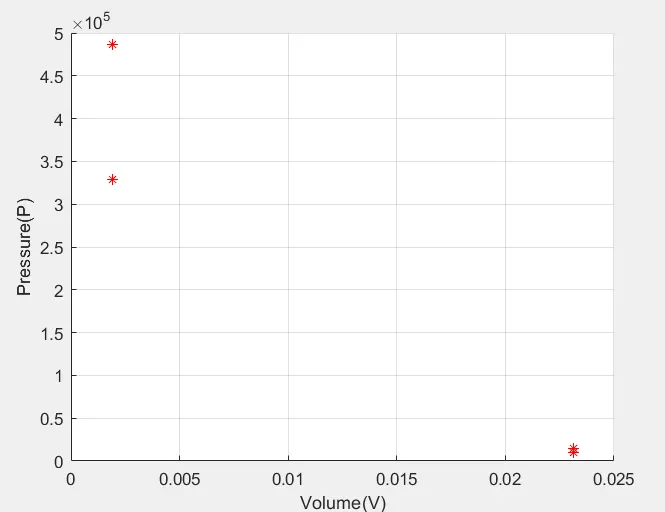
5. Using all the data, we first plot the four points in the PV graph. This is done using the ’plot’ command.
6. For plotting all the points in the same graph, we first open a figure window and use ‘hold on’ command to plot the points in this figure.
7. Now for joining these points to make a PV diagram, we create a function to calculate the swept volume by the formula mentioned above.
8. We call this function in our main program and store the values in a specific array. We calculate corresponding pressure array using appropriate equation.
9. Using ‘plot’ command, the PV diagram is completed by joining the four state points.
10. For thermal efficiency, write the formula and store the value in a variable.

CODE:

clear all 
close all
clc

% inputs
gamma = 1.4;
t3 = 2400;

% state variables 
p1 = 10135;
t1 = 600;

% Engine parameters
bore = 0.3;
stroke = 0.3;
con_rod = 0.4;
cr = 12;

v_swept = (pi/4)*bore^2*stroke;
v_clearance = v_swept/(cr-1);

v1 = v_swept + v_clearance;
v2 = v_clearance;

% state variables at point 2
p2 = p1*(cr^gamma);    % (v1/v2) = cr

t2 = (p2*v2*t1)/(p1*v1);     % p1v1/t1 = p2v2/t2

constant_c = p1*(v1^gamma);
V_compression = engine_kinematics(bore, stroke, con_rod, cr, 180, 0);
P_compression = constant_c./(V_compression.^gamma);

% state variables at point 3
v3 = v2;

p3 = p2*t3/t2;      % p2t2 = p3t3

constant_c = p3*v3^gamma;
V_expansion = engine_kinematics(bore, stroke, con_rod, cr, 0, 180);
P_expansion = constant_c./(V_expansion.^gamma);

%state variables at poiint 4
v4 = v1;

p4 = p3*((v3/v4)^gamma);     % p3.v3^gamma = p4.v4^gamma

t4 = (p4*v4*t3)/(p3*v3);


% plotting in P-V graph
figure(1)
hold on
plot(v1,p1,'*','color','r')
plot(V_compression, P_compression)
plot(v2,p2,'*','color','r')
plot([v2 v3], [p2 p3],'color','b')
plot(v3,p3,'*','color','r')
plot(V_expansion, P_expansion)
plot(v4,p4,'*','color','r')
plot([v4 v1], [p4 p1],'color','b')
xlabel('Volume(V)')
ylabel('Pressure(P)')


% thermal efficiency of otto cycle
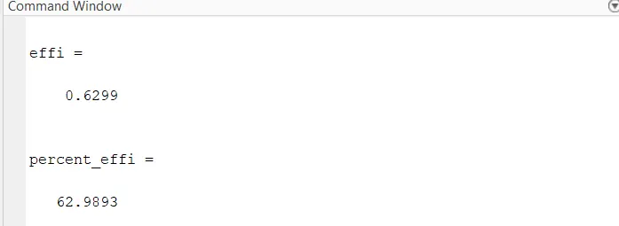
effi = 1 + (t1 - t4)/(t3 - t2)

percent_effi = effi*100

FUNCTION CODE:

function [V] = engine_kinematics(bore, stroke, con_rod, cr, start_crank, end_crank)

v_s = (pi/4)*bore^2*stroke;
v_c = v_s/(cr-1);

a = stroke/2;
R = con_rod/a;



% breaking the formula in parts

theta  = linspace(start_crank, end_crank, 180);

term1 = 0.5*(cr-1);
term2 = R + 1 - cosd(theta);
term3 = (R^2 - sind(theta).^2).^0.5;

V = (1 + term1*(term2 - term3))*v_c;
end

OUTPUT:

PLOTTED POINTS:

PV DIAGRAM:

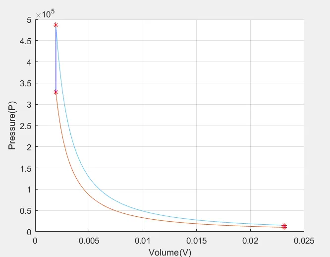
CONCLUSION:1. We have plotted the state points in a PV graph and also plotted a PV diagram for the given Otto Cycle.

2. We have studied how to solve Otto Cycle and plot graphs for it. In this way we can solve any ‘Air Standard Cycle’ using MATLAB.