Polynomial Curve Fitting using MATLAB

AIM: To perform curve fitting operations on the given dataset using MATLAB.

OBJECTIVES:

1. Write code to fit a linear and cubic polynomial for the Cp data.
2. Plot the linear and cubic fit curves along with the raw data points. Title and axes labels are a must, legends could be shown if necessary.
3. Write a code to show split-wise method.
4. Explain the parameters used to measure the fitness characteristics for both the curves.

INTRODUCTION:

Curve Fitting: Curve Fitting is the process of creating a curve or mathematical function that has the best fit to a series of data points.

We use polynomial equations for creating a function for given data sets and plot the graph according to these equations.

Fitting functions to data points:

1. The first degree polynomial equation

`y=ax+b`

is a line with slope a. A line will connect any two points, so a first-degree polynomial equation is an exact fit through any two points with distinct x coordinates.

2. If the order of the equation is increased to a second-degree polynomial, the following results:

`y = ax^2 + bx + c`

This will exactly fit a simple curve to three points.

2. If the order of the equation is increased to a third-degree polynomial, the following is obtained:

`y= ax^3 + bx^2 + cx + d`

This will exactly fit four points.

PROCEDURE:

I. For linear and cubic curve fitting:

1. Firstly, load the given data set and store the values in a variable. We have two values “temperature” and “specific heat”. Create separate arrays for both and store the values in them.
2. Open a figure window and plot the curve for original data.
3. For curve fitting we use two main functions named ‘polyfit’ and ‘polyval’.

‘polyfit’ is used to create coefficients for a polynomial of specific degree.

‘polyval’ is used to evaluate the polynomial for each value of the independent variable from the given data set.

4. We define the degree of freedom ‘1’ for plotting linear curve. And write ‘3’ for cubic curve fitting.
5. Use ‘plot’ command to plot the curve. We use different figure windows to plot ‘linear fit’ and ‘cubic fit’ to get separate graphs for both in order to compare more easily.
6. Give proper name to both the figures using ‘title’ command. Give suitable labels to the axes.

CODE:

clear all
close all
clc

%loading data and storing values in seperate arrays
cp_data = load('data');

cp = cp_data(:,2);
temp = cp_data(:,1);

figure(1)
hold on
plot(temp,cp,'linewidth',3)

%linear curve fitting
cp_coeff_linear = polyfit(temp,cp,1);
CP1 = polyval(cp_coeff_linear, temp);
plot(temp,CP1,'color','r','linewidth',3)
title('Linear Curve Fitting')
xlabel('Temperature [K]')
ylabel('Specific Heat [KJ/Kmol-K]')
legend('Original Dataset', 'Curve Fit')
grid on

%cubic curve fitting
figure(2)
hold on
plot(temp,cp,'linewidth',3)

cp_coeff_cubic = polyfit(temp,cp,3);
CP3 = polyval(cp_coeff_cubic,temp);
plot(temp,CP3,'color','r','linewidth',3)
title('Cubic Curve Fitting')
xlabel('Temperature [K]')
ylabel('Specific Heat [KJ/Kmol-K]')
legend('Original Dataset', 'Curve Fit')
grid on

PLOTS:

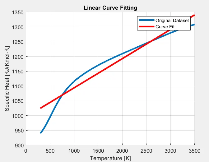
1. Linear Curve Fit:

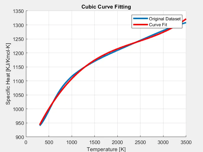
2. Cubic Curve Fit:

II. For Split-wise method:

1. In split-wise method, we divide the given data set into suitable parts and fit curves in those parts.
2. Here we divide the given set of data in five equal parts.
3. Create polynomial coefficients for these five parts. And create five different polynomials.
4. Then we plot these five curves in the same figure window where we also plot the original data curve for comparison purpose.
5. Using this method reduces the error, which means the difference between original and curve fitted values is minimised.

CODE:

%dividing the temp range and cp range
cp1 = cp(1:640);
cp2 = cp(641:1280);
cp3 = cp(1281:1920);
cp4 = cp(1921:2560);
cp5 = cp(2561:3200);

temp1 = temp(1:640);
temp2 = temp(641:1280);
temp3 = temp(1281:1920);
temp4 = temp(1921:2560);
temp5 = temp(2561:3200);

%creating polynomial for different range
cp_coeff1 = polyfit(temp1,cp1,3);
cp_coeff2 = polyfit(temp2,cp2,3);
cp_coeff3 = polyfit(temp3,cp3,3);
cp_coeff4 = polyfit(temp4,cp4,3);
cp_coeff5 = polyfit(temp5,cp5,3);

CP1 = polyval(cp_coeff1, temp1);
CP2 = polyval(cp_coeff2, temp2);
CP3 = polyval(cp_coeff3, temp3);
CP4 = polyval(cp_coeff4, temp4);
CP5 = polyval(cp_coeff5, temp5);

%plotting the functions
figure(3)
plot(temp,cp,'linewidth',3)
hold on
plot(temp1,CP1,'color','r','linewidth',2)
plot(temp2,CP2,'color','r','linewidth',2)
plot(temp3,CP3,'color','r','linewidth',2)
plot(temp4,CP4,'color','r','linewidth',2)
plot(temp5,CP5,'color','r','linewidth',2)

title('Cubic Split-wise Curve Fitting')
xlabel('Temperature [K]')
ylabel('Specific Heat [KJ/Kmol-K]')
legend('Original Dataset', 'Curve Fit')
grid on

PLOT:

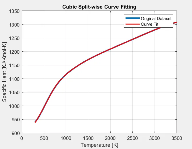
Split-wise curve fitting:

FITNESS OF THE CURVE:

Let us assume our function is ‘y = f(x)’.

We have ‘n’ number of data points.

For i^th data point the value of function is ‘f(x(i))’ and the actual value of the output is ‘y(i)’.

There are four parameters that decide the goodness of the fit of our curve.

1. Squared sum of errors (SSE):

The error at any point, say i, iis given by:

Error = │y(i) – f(x(i))│

Now SSE is the sum of square of all the errors, and is calculated as:

If the value of SSE is less, say close to zero, the curve is said to be a good fit.

2. R-square:

R-square is the measure of how successful the fit is and how successfully explains the variation of our data. In other words, if the value of R is greater, then our curve is said to be in good fit.

The value of R is calculated by:

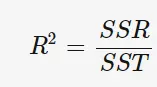
Where, SSR = sum of squares of regression

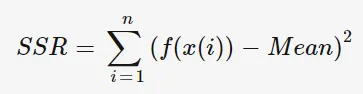
SST = SSR + SSE

R acquires values between 0 to 1. So, the fit is better if R has value near to 1 and the fit is if the value is near 0.

3. Adjusted R-square:

When a variable is introduced in our system, it will have following effects:

1. Its value contributes to the output, if it is ‘Significant Dependent Variable’.
2. Its value does not affect the output, if it is ‘Insignificant Dependent Variable’.

When an insignificant variable is introduced, the Adjusted R-square takes the values according to the no. of total data points and number of dependent variables that actually contributes to the value of output.

Adjusted R-square is formulated as:

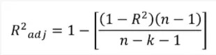
Where, n = number of data points

k = number of independent variables

4. Root Mean Square Error (RMSE):

RMSE is also known as fit standard error and the standard error of regression.

Using these four parameters, we can determine the goodness of the fit. If the value of R-square is greater than 0.95, the curve fit is assumed to be good.

1. How to make a curve fit perfectly?

For a perfect fit, the value of R-square needs to be exactly equal to 1.

for this, the value of SSE should be equal to zero.

2. How to get the best fit?

When we create a polynomial function for curve fitting, the degree of that polynomial plays an important role in making the fit good or bad.

If the degree of the polynomial is higher, then the curve fit is better.

Here we use a third-degree polynomial which is a better fit than a quadratic function.

When a polynomial of higher order is created and plotted, it fits better than the cubic curve fit.

Hence to get the best, the degree of the polynomial can be increased to the appropriate high value.

3. What could be done to improve the cubic fit?

A cubic curve is not the best fit as we can observe in the plot. But the fit can be improved by dividing the set of data into small data.

Here we split the given data into 5 equal parts and create seperate polynomial functions for these five data sets. Plotting these functions in one graph will show more accuracy than the single cubic curve function and hence minimising the error.

CONCLUSION:

1. From the plot of 'Linear Curve Fit', it is clear that line fits only two points from the data set. Hence it is not a good for our data points.

2. 'Cubic Curve Fit' figure shows that the fit is far better than the linear fit. This curve fits most of the data points in our data set.

3. When we split our data set into smaller sets and plot the funciton according the new data sets, the cubic curve is improved to a good extent. The curve fits more data points than the cubic curve for single data set that we plotted before.

We have studied 'Curve Fitting' and how to use MATLAB for fittting curves for given data sets.

REFERENCES:

1. https://en.wikipedia.org/wiki/Curve_fitting
2. https://statisticsbyjim.com/regression/curve-fitting-linear-nonlinear-regression/
3. https://skill-lync.com/projects/Curve-Fitting-and-criterion-to-choose-best-fit-41860