Vehicle Dynamics - Combined Slip Brush Tire Model using MATLAB

AIM: To write a MATLAB code for plotting the combined slip tire model.

OBJECTIVES: To plot a graph showing effect of different slip angles on Lateral Force v/s Longitudinal Force relationship.

GIVEN DATA:

GOVERNING EQUATIONS: In combined slip model, the tire is under both the lateral and longitudinal forces and is deterbined as follows-

i) Adhesion region

Cornering stiffness, `C_(alpha) = 1/2*K_(t_y)*l_t^2`

Longitudinal stiffness, `C_s = 1/2*K_(t_x)*l_t^2`

Longitudinal force, `F_x = (C_s*i_s)/(1-i_s)`

Lateral force, `F_y = (C_(alpha)*tan(alpha))/(1-i_s)`

where,

`i_s ->`slip ratio

`l_t ->`contact patch length

`K_(t_x) ->`tire tangential stiffness

`K_(t_y) ->`tire lateral stiffness

ii) Critical length

`l_c = (mu*F_z*(1-i_s)*l_t)/(2*sqrt((C_s*i_s)^2+(C_(alpha)*tan(alpha))^2`

where,

`mu ->`coefficient of friction

`F_z ->`Normal load

iii) Sliding region

Longitudinal force, `F_x = (mu*F_z*C_s*i_s)/sqrt((C_s*i_s)^2+(C_(alpha)*tan(alpha))^2)[1-(mu*F_z*(1-i_s))/(4*sqrt((C_s*i_s)^2+(C_(alpha)*tan(alpha))^2))]`

Lateral force, `F_y = (mu*F_z*C_s*tan(alpha))/sqrt((C_s*i_s)^2+(C_(alpha)*tan(alpha))^2)[1-(mu*F_z*(1-i_s))/(4*sqrt((C_s*i_s)^2+(C_(alpha)*tan(alpha))^2))]`

SOLUTION:

MATLAB Code:

clear all
close all
clc

%inputs
Fz = 4000;      %normal load in N
mu = 0.85;      %Coeff. of friction
lt = 0.2;       %lenght of contact patch in m
Kt_t = 3.5e6;       %tire tangential stiffness per unit length in N/m^2
Kt_l = 2.5e6;       %tire lateral stiffness per unit length in N/m^2

%cornering stiffness
Ca = 0.5*Kt_l*lt^2;     %cornering stiffness
Cs = 0.5*Kt_t*lt^2;     %longitudinal stiffness

for i = 2:2:10
    alpha = i*pi/180;       %slip angle
    for j = 1:101
        is(j) = (j-1)*0.01;      %slip ratio
        temp(j) = ((Cs*is(j))^2 + (Ca*tan(alpha))^2)^0.5;    
        lc(j) = mu*Fz*(1-is(j))*lt/(2*temp(j));      %critcal length
        
        if lt <= lc
            Fx(j) = Cs*is(j)/(1-is(j));
            Fy(j) = Ca*tan(alpha)/(1-is(j))    
        else
            Fx(j) = (mu*Fz*Cs*is(j)/temp(j))*((1-mu*Fz*(1-is(j))/(4*temp(j))));
            Fy(j) = (mu*Fz*Ca*tan(alpha)/temp(j))*((1-mu*Fz*(1-is(j))/(4*temp(j))));
        end
    end
    
    %plotting curves for each iteration
    figure(1)
    hold on
    plot(Fx,Fy,'linewidth',2)
  
end

%plot properties
    title('Lateral Force v/s Longitudinal Force')
    xlabel('Longitudinal Force (N)')
    ylabel('Latera Force (N)')
    legend('2 deg','4 deg','6 deg','8 deg','10 deg')
    grid on

    saveas(1,'combined_slip','jpeg')

OUTPUT:

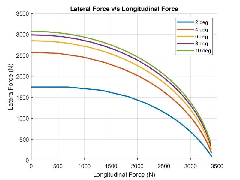
Inference from the plot:

1. As the longitudinal force increases, the lateral force decreases.

2. The magnitudes of both the force at any given instance is not equal. Hence, the graph is elliptical in nature.

3. Lateral force increases with increase in slip angle.

CONCLUSION: The plot for effect of slip angle on Fx v/s Fy is plotted successfully using MATLAB.

AIM: To calculate effective stiffness values for different slip ratios

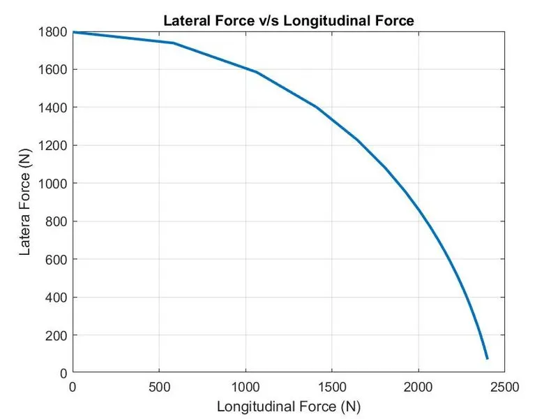
OBJECTIVE: Write a MATLAB script to calculate effective stiffness and plot the following graphs-

i) Lateral force v/s Longitudinal force

ii) Effective cornering stiffness v/s Slip ratio

GIVEN DATA:

GOVERNING EQUATION:

Effective cornering stiffness, `C_(alpha_(eff)) = F_y/(alpha)`

SOLUTION:

MATLAB code:

clear all
close all
clc

%inputs
Fz = 3000;      %Normal load in N
mu = 0.8;      %coeff. of frcition
lt = 0.2;       %length of contact patch in m
Kt_t = 4.0e6;       %tire tangential stiffness per unit length in N/m^2
Kt_l = 2.275e6;       %tire lateral stiffness per unit length in N/m^2
alpha = 3.0;        %slip angle in deg

%cornering stiffness
Ca = 0.5*Kt_l*lt^2;     %cornering stiffness
Cs = 0.5*Kt_t*lt^2;     %longitudinal stiffness

is = [0,0.15,1.0];      %given slip ratios
alpha = alpha*pi/180;

%loop for effective Ca values
for i = 1:length(is)
        temp(i) = ((Cs*is(i))^2 + (Ca*tan(alpha))^2)^0.5;    
        lc(i) = mu*Fz*(1-is(i))*lt/(2*temp(i));      %critcal length
        
        if lt <= lc
            Fx(i) = Cs*is(i)/(1-is(i));
            Fy(i) = Ca*tan(alpha)/(1-is(i));
            Ca_eff(i) = Fy(i)/alpha;
        else
            Fx(i) = (mu*Fz*Cs*is(i)/temp(i))*((1-mu*Fz*(1-is(i))/(4*temp(i))));
            Fy(i) = (mu*Fz*Ca*tan(alpha)/temp(i))*((1-mu*Fz*(1-is(i))/(4*temp(i))));
            Ca_eff(i) = Fy(i)/alpha;
        end
    
end
display([is])
display([Ca_eff])

%loop for plotting graphs
for j = 1:101
        is(j) = (j-1)*0.01;      %slip ratio
        temp(j) = ((Cs*is(j))^2 + (Ca*tan(alpha))^2)^0.5;    
        lc(j) = mu*Fz*(1-is(j))*lt/(2*temp(j));      %critcal length
        
        if lt <= lc
            Fx(j) = Cs*is(j)/(1-is(j));
            Fy(j) = Ca*tan(alpha)/(1-is(j));
            Ca_eff(j) = Fy(j)/alpha;
        else
            Fx(j) = (mu*Fz*Cs*is(j)/temp(j))*((1-mu*Fz*(1-is(j))/(4*temp(j))));
            Fy(j) = (mu*Fz*Ca*tan(alpha)/temp(j))*((1-mu*Fz*(1-is(j))/(4*temp(j))));
            Ca_eff(j) = Fy(j)/alpha;
        end
end
    
%plotting the graphs

figure(1)
plot(Fx,Fy,'linewidth',2)
title('Lateral Force v/s Longitudinal Force')
xlabel('Longitudinal Force (N)')
ylabel('Latera Force (N)')
grid on

figure(2)
plot(is,Ca_eff,'linewidth',2)
title('Effective cornering stiffness v/s Slip ratio')
xlabel('Slip ratio')
ylabel('Effective cornering stiffness')
grid on

saveas(1,'combined_slip_2b_1','jpeg')
saveas(2,'combined_slip_2b_2','jpeg')

OUTPUT:

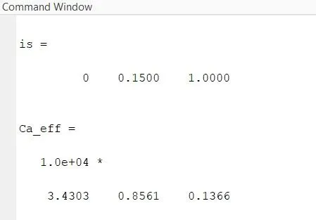
Final deliverables-

Slip ratio	Effective cornering stiffness
0	3.4303E4
0.15	0.8561E4
1	0.1336E4

PLOTS:

Plot 1:

Plot 2:

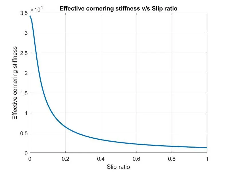
Inference from the plot:

From plot 2, we can see that the effective cornering stiffness decreases with increase in slip ratio. That means, there will be less complaince with greater difference in the rotaional and translational speed of the tire.

CONCLUSION: The values of effective cornering stiffnes for different values of slip ratios have been dtermined using an errorless MATLAB script.