FINAL INDEPENDENT PROJECT
FINAL INDEPENDENT PROJECT
TITLE:
INFLUENCE OF PERMANENT MAGNET DC MOTOR PARAMETERS ON STARTING TRANSIENT PROCESS
AIM:
To calculate the startup characteristics of Permanent Magnet DC Motor and allow to show the influence of motor parameters on the electromechanical transient process.
Introduction
Permanent Magnet DC Motor or PMDC Motor | Working Principle Construction
In a DC motor, an armature rotates inside a magnetic field. The basic working principle of a DC motor is based on the fact that whenever a current-carrying conductor is placed inside a magnetic field, there will be a mechanical force experienced by that conductor.
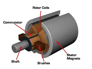
Fig. 1. Permanent magnet DC motor construction
All kinds of DC motors work in this principle only. Hence for constructing a DC motor, it is essential to establish a magnetic field. The magnetic field is obviously established by means of a magnet. The magnet can be any type, i.e. it may be an electromagnet or it can be a permanent magnet. When a permanent magnet is used to create a magnetic field in a DC motor, the motor is referred as a permanent magnet DC motor or PMDC motor. These types of motor are essentially simple in construction. These motors are commonly used as a starter motor in vehicles, windshield wipers, washers, for blowers used in heaters and air conditioners, to raise and lower windows, it also extensively used in toys.
The processes occurring when the rotational speed of electric motors and electric drives varies are called electromechanical transient processes.
In general, the transient process in a DC machine is described by a system of differential equations for the armature winding and the excitation winding, supplemented by the equation of the electromagnetic torque (the equation of torque equilibrium or the equation of armature motion).
Dynamic Model of a Permanent Magnet DC Motor
Mathematical Model
The goal in the development of the mathematical model is to relate the voltage applied to the armature to the rotational speed of the motor. Two balance equations can be developed by considering the electrical and mechanical characteristics of the system.
Electrical Characteristics
The equivalent electrical circuit of a dc motor is illustrated in Fig. 2. It can be represented by a voltage source (Ua) across the coil of the armature. The electrical equivalent of the armature coil can be described by an inductance (La) in series with a resistance (Ra) in series with an induced voltage (e) which opposes the voltage source. The induced voltage is generated by the rotation of the electrical coil through the fixed flux lines of the permanent magnets. This voltage is often referred to as the back emf (electromotive force).
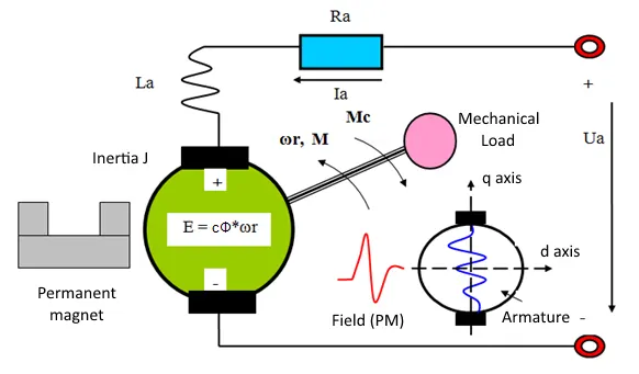
Fig. 2. An electrical representation of a permanent magnet DC motor
A differential equation for the equivalent circuit can be derived by using Kirchoff’s voltage law around the electrical loop. Kirchoff’s voltage law states that the sum of all voltages around a loop must equal zero, or

where
 is the voltage drop across the resistor, according to Ohm's law, is the armature current,
 is the voltage across the inductor is proportional to the change of current through the coil with respect to time,
e = сФω is the back emf,
where сФ is the motor voltage constant determined by the flux density of the permanent magnets, the reluctance of the iron core of the armature and the number of turns of the armature winding,
ω is the rotational velocity of the rotor (armature).
Mechanical Characteristics
Performing an energy balance on the system, the sum of the torques of the motor must equal zero. Therefore,

where T is the electromagnetic torque,
 is the torque of the mechanical load,
 is the torque due to rotational acceleration of the rotor,
is the torque produced from the velocity of the rotor, and
J is the inertia of the rotor and the equivalent mechanical load.
The electromagnetic torque T is proportional to the current through the armature winding and can be written as

The instantaneous value of the current ia is found from the expression for the electromagnetic torque:

The differential equation for angular speed


And:

The equation for armature voltage can be rewritten in the form:

After the transformations, we obtain:

We obtain the ordinary differential equation of second order for rotational speed.
The differential equation for armature current will be:

Initialization of the DC motor parameters:
DC motor parameters can be taken from the Parameters for servomotor 3PI12.18 (695 W) are:
Ra = 0.53;                                    % armature winding resistance, Ohm
La = 0.0038;                                  % armature winding inductance , H
J = 0.0051;                                   % armature inertia, kg*m^2
U = 155;                                      % supply voltage, V
Tem = 0.008;                                  % electromechanical time constant, s
Mc = 7;                                       % load torque, N*m
cF = sqrt(Ra*J/Tem);                          % calculation of c*Ф, where c is the back-EMF coefficient and Ф is a magnetic flux
Ta = La/Ra;                                   % electromagnetic time constant, s
To solve the system of equations, it is necessary to create an M-file, in which the vector-function f(y,t) is calculated.
function dwdt = difsys(~, w, Ra, La, J, Mc, U, cF)
%where
%w(1) -> w(t) (the required function)
%w(2) -> dw/dt (derivative)
%w(3) -> i(t) (armature current)
%dwdt(1) -> dw/dt (the first derivative)
%dwdt(2) -> d2w/dt2 (the second derivative)
%dwdt(3) -> (the first currrent derivative)

dwdt = zeros(3,1);
dwdt(1) = w(2);                                               %Right hand part; the first derivative of speed
dwdt(2) = -(Ra/La)*w(2)-cF^2/La/J*w(1)+U*cF/La/J-Ra*Mc/La/J;  %Right hand part of the differential equation(1)
dwdt(3) = -w(3)*Ra/La-cF*w(1)/La+U/La;                        %Right hand part of the differential equation(3)
end
Now we are writing a code for the main program in MATLAB;
clear all;
close all;
clc;


Ra = 0.53;                                    % armature winding resistance, Ohm
La = 0.0038;                                  % armature winding inductance , H
J = 0.0051;                                   % armature inertia, kg*m^2
U = 155;                                      % supply voltage, V
Tem = 0.008;                                  % electromechanical time constant, s
Mc = 7;                                       % load torque, N*m
cF = sqrt(Ra*J/Tem);                          % calculation of c*Ф, where c is the back-EMF coefficient and Ф is a magnetic flux
Ta = La/Ra;                                   % electromagnetic time constant, s

tspan = [0 0.15];                                % time interval
w0 = [0 0 0];                                    % initial values of functions and derivatives
[T, W] = ode45(@(t,w)difsys(t, w, Ra, La, J, Mc, U, cF),tspan,w0); % ODE solution

W(:,1)=30/pi*W(:,1);                          % recalculation of speed from rad/s to rpm
[T,W];


figure(1);
hold on
yyaxis left
plot(T, W(:,1))
plot(T, W(:,2))
xlabel('t, s')                                               % name horizontal axis (x)
ylabel('n, rpm; d\omega/dt, 1/s^2')                          % name left vertical axis (y)

yyaxis right
ylim([-50,200])
plot(T, W(:,3))
xlabel('t, s')                                               % name horizontal axis (x)
ylabel('Armature current, A')                                % name right vertical axis (y)
hold off
grid on
title('Transient plots')                                     % add plot name
legend('rotational speed n(t)','speed derivative d\omega/dt', 'armature current i(t)')  % add legend
fprintf ('Tem/Ta = %g ', Tem/Ta);

figure(2);
plot(T,W(:,3))
grid on                                       % enable grid
title('Armature current')                     % add plot name
legend('armature current i(t)')               % add legend
xlabel('t, s')                                % name horizontal axis (x)
ylabel('Armature current, A')                 % name vertical axis (y)

figure(3);
plot(T,W(:,1))
grid on                                       % enable grid
title('Rotational speed')                     % add plot name
legend('rotational speed n(t)')               % add legend
xlabel('t, s')                                % name horizontal axis (x)
ylabel('Rotational speed, rpm')               % name vertical axis (y)

Mem = W(:,3)*cF;
figure(4);
plot(T, Mem)
grid on                                       % enable grid
title('Electromagnetic torque')               % add plot name
legend('torque, Mem(t)')                      % add legend
xlabel('t, s')                                % name horizontal axis (x)
ylabel('Torque, N*m')                         % name vertical axis (y)

% motor parameters and rated values
Ra = 0.53;                                    % armature winding resistance, Ohm
La = 0.0038;                                  % armature winding inductance, H
J = 0.0051;                                   % armature inertia, kg*m^2
U = 155;                                      % supply voltage, V
Tem = 0.008;                                  % electromechanical time constant, s
Mc = 7;                                       % load torque, N*m
cF = sqrt(Ra*J/Tem);                          % calculation of c*Ф, where c is the back-EMF coefficient and Ф is magnetic flux
Ta = La/Ra;                                   % electromagnetic time constant, s

Rvar=[0.5 1 2]*Ra;                            % Ra variation, e.g. 0.5*Ra or 2*Ra
figure(5);
for k = 1:length(Rvar)
    Ra = Rvar(k);
    tspan = [0 0.15];
    w0 = [0 0 0];
    [T, W] = ode45(@(t,w)difsys(t, w, Ra, La, J, Mc, U, cF),tspan,w0);

    W(:,1) = 30/pi*W(:,1);
    Mem = W(:,3)*cF;
    hold on;
    subplot(2,1,1);
    plot(T,W(:,1)); title('Influence of the armature resistance on the transient process');
    xlabel('t, s'); ylabel('Rotational speed, rpm'); grid on;
    hold on;
    subplot(2,1,2);
    plot(T,W(:,3)); xlabel('t, s'); ylabel('Armature current, A'); grid on;
end
hold off;

subplot(2,1,1); title(legend(num2str(Rvar'),'Location', 'southeast'),'Ra, Ohm');
subplot(2,1,2); title(legend(num2str(Rvar'),'Location', 'northeast'),'Ra, Ohm');
Tem = Rvar.*J/cF^2;
Ta = La./Rvar;
ratio = Tem./Ta;

% motor parameters and rated values
Ra = 0.53;                                    % armature winding resistance, Ohm
La = 0.0038;                                  % armature winding inductance, H
J = 0.0051;                                   % armature inertia, kg*m^2
U = 155;                                      % supply voltage, V
Tem = 0.008;                                  % electromechanical time constant, s
Mc = 7;                                       % load torque, N*m
cF = sqrt(Ra*J/Tem);                          % calculation of c*Ф, where c is the back-EMF coefficient and Ф is magnetic flux
Ta = La/Ra;                                   % electromagnetic time constant, s

cFvar=[0.8 1 2]*cF;                           % cФ variation, e.g. 0.5*cФ or 1.5*cФ
figure(6);
for k = 1:length(cFvar)
    cF = cFvar(k);
    tspan = [0 0.15];
    w0 = [0 0 0];
    [T, W] = ode45(@(t,w)difsys(t, w, Ra, La, J, Mc, U, cF),tspan,w0);
    W(:,1)=30/pi*W(:,1);
    Mem=W(:,3)*cF;
    hold on;
    subplot(2,1,1);
    plot(T,W(:,1));title('Influence of the excitation flux on the transient process');
    xlabel('t, s'); ylabel('Rotational speed, rpm'); grid on;

    hold on;
    subplot(2,1,2);
    plot(T,W(:,3));xlabel('t, s'); ylabel('Armature current, A'); grid on;
end
hold off;

subplot(2,1,1); title(legend(num2str(cFvar'),'Location', 'southeast'), 'cФ');
subplot(2,1,2); title(legend(num2str(cFvar'),'Location', 'northeast'), 'cФ');

% motor parameters and rated values
Ra = 0.53;                                    % armature winding resistance, Ohm
La = 0.0038;                                  % armature winding inductance, H
J = 0.0051;                                   % armature inertia, kg*m^2
U = 155;                                      % supply voltage, V
Tem = 0.008;                                  % electromechanical time constant, s
Mc = 7;                                       % load torque, N*m
cF = sqrt(Ra*J/Tem);                          % calculation of c*Ф, where c is the back-EMF coefficient and Ф is magnetic flux
Ta = La/Ra;                                   % electromagnetic time constant, s

Uvar=[0.5 1 1.5]*U;                           % U variation, e.g. 0.5*U or 1.5*U
figure(7);
for k = 1:length(Uvar)
    U = Uvar(k);
    tspan = [0 0.15];
    w0 = [0 0 0];
    [T, W] = ode45(@(t,w)difsys(t, w, Ra, La, J, Mc, U, cF),tspan,w0);
    W(:,1)=30/pi*W(:,1);
    Mem=W(:,3)*cF;
    hold on;
    subplot(2,1,1);
    plot(T,W(:,1));title('Influence of the supply voltage on the transient process');
    xlabel('t, s'); ylabel('Rotational speed, rpm'); grid on;

    hold on;
    subplot(2,1,2);
    plot(T,W(:,3));xlabel('t, s'); ylabel('Armature current, A'); grid on;
end
hold off;

subplot(2,1,1); title(legend(num2str(Uvar'),'Location', 'southeast'), 'U, V');
subplot(2,1,2); title(legend(num2str(Uvar'),'Location', 'northeast'), 'U, V');
Differential equations solution
Integration of ordinary differential equations is performed by the functions ode23 and ode45. They can be used both for a numerical solution (integration) of simple differential equations, and for modelling complex dynamical systems, i.e. systems whose behavior can be described by a set of ordinary differential equations.
It is known that any system of ordinary differential equations (ODE) can be represented as a system of first-order equations in the Cauchy form:

where y is the vector of state variables (phase variables of the system); t - argument (usually - time); f is a nonlinear vector-function of the state variables y and the argument t.
Call of the procedures has the following syntax:
[t, y] = ode23 (‘<function name>’, tspan, y0, options)
[t, y] = ode45 (‘<function name>’, tspan, y0, options),
where the parameters used have the following meaning: <function name> is a character string representing the name of the M-file, in which the vector function f(y,t) is calculated, ie, the right-hand parts of the ODE system; y0 is a vector of initial values of state variables; t is an array of calculated values of the argument corresponding to the steps of integration; y is the matrix of the integrated values of the phase variables, in which each column corresponds to one of the state variables, and the line contains the values of the state variables corresponding to the integration step; tspan is a row vector [t0 tfinal], containing two values: t0 - initial and tfinal - final value of the argument; options is a string of parameters that determine the values of the permissible relative and absolute integration errors.
Options can be omitted. Then, by default, the permissible relative error of integration is assumed to be 1⋅10^-3, and absolute error (for any of the state variables) is 1⋅10^-6. If these values do not suit the user then the new values of permissible errors have to be set before calling the procedure of numerical integration, using the odeset procedure in this way:
options = odeset ('RelTol',1e-4,'AbsTol',[1e-4 1e-4 1e-5]).
The parameter RelTol determines the relative error of numerical integration over all phase variables simultaneously, and AbsTol is a vector-string consisting of absolute admissible errors of numerical integration for each of the phase variables.
The function ode23 integrates numerically by the Runge-Kutta numerical method of the second order, and, by means of the third-order method, controls the relative and absolute integration errors at each step and changes the magnitude of the integration step so as to provide the specified limits of integration errors.
For the function ode45, the main method of integration is the fourth-order Runge-Kutta method, and the step size is controlled by the 5th order method. [6]
To solve differential equations and systems in MATLAB, the following functions are provided:
ode45 (f, interval, X0, [options])
ode23 (f, interval, X0, [options])
The input parameters of these functions are:
- f— vector function for calculating the right-hand side of the equations of the system of differential equations;
- interval— an array of two numbers that defines the interval of integration of a differential equation or system;
- Х0— vector of initial conditions of the system of differential equations;
- options— control parameters of the solution of a differential equation or system.
All functions return:
- array Т— the coordinates of the grid nodes in which the solution is sought;
- matrix X, whose i-th column is the value of solution vector-function at the node Ti.
In the problem posed, it is necessary to solve a system of three differential equations:
- the equation for the first derivative of the speed;
- the equation for the second derivative of the speed;
- the equation for the current derivative.
tspan = [0 0.15];                                % time interval
w0 = [0 0 0];                                    % initial values of functions and derivatives
[T, W] = ode45(@(t,w)difsys(t, w, Ra, La, J, Mc, U, cF),tspan,w0); % ODE solution

W(:,1)=30/pi*W(:,1);                             % recalculation of speed from rad/s to rpm
[T,W];
The solution shall be:
- array T — vector-column of the calculated time;
- array W — matrix of three columns, where the 1st column is the value of the rotational speed, the second is the first derivative of the rotation frequency, the third is the current of the armature.
All values of the first column are also recalculated to obtain the speed values in revolutions per minute (rpm).
Now we can plot the graphs of the transient process, where the horizontal axis is the solution vector T and the vertical axis is the values of the found functions.
figure(1);
hold on
yyaxis left
plot(T, W(:,1))
plot(T, W(:,2))
xlabel('t, s')                                               % name horizontal axis (x)
ylabel('n, rpm; d\omega/dt, 1/s^2')                          % name left vertical axis (y)

yyaxis right
ylim([-50,200])
plot(T, W(:,3))
xlabel('t, s')                                               % name horizontal axis (x)
ylabel('Armature current, A')                                % name right vertical axis (y)
hold off
grid on
title('Transient plots')                                     % add plot name
legend('rotational speed n(t)','speed derivative d\omega/dt', 'armature current i(t)')  % add legend
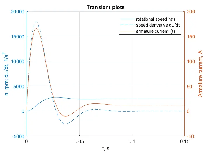
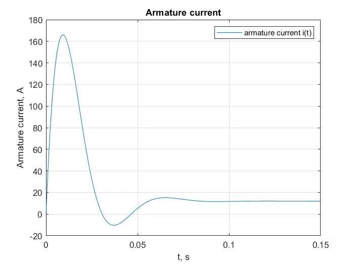
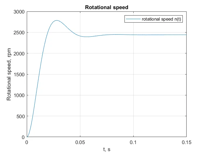
Due to the fact that the armature circuit has an inductance (), the current in the armature circuit does not instantaneously reach the instantaneous value of, but approaches it exponentially

When the current  , at the time instant
  , reaches the value corresponding to the load torque

the motor armature will start to rotate, and the EMF will be induced in its winding e = cωΦ. The current rise will slow down. At time , the current reaches the maximum. At this moment, the angular acceleration
 is maximal. Then the current decreases to the value, and the angular speed approaches its steady-state value.
figure(2);
plot(T,W(:,3))
grid on                                       % enable grid
title('Armature current')                     % add plot name
legend('armature current i(t)')               % add legend
xlabel('t, s')                                % name horizontal axis (x)
ylabel('Armature current, A')                 % name vertical axis (y)
figure(3);
plot(T,W(:,1))
grid on                                       % enable grid
title('Rotational speed')                     % add plot name
legend('rotational speed n(t)')               % add legend
xlabel('t, s')                                % name horizontal axis (x)
ylabel('Rotational speed, rpm')               % name vertical axis (y)
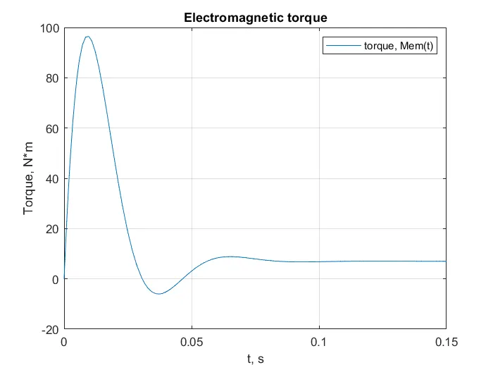
Mem = W(:,3)*cF;
figure(4);
plot(T, Mem)
grid on                                       % enable grid
title('Electromagnetic torque')               % add plot name
legend('torque, Mem(t)')                      % add legend
xlabel('t, s')                                % name horizontal axis (x)
ylabel('Torque, N*m')                         % name vertical axis (y)
The influence of the armature resistance on the transient process
% motor parameters and rated values
Ra = 0.53;                                    % armature winding resistance, Ohm
La = 0.0038;                                  % armature winding inductance, H
J = 0.0051;                                   % armature inertia, kg*m^2
U = 155;                                      % supply voltage, V
Tem = 0.008;                                  % electromechanical time constant, s
Mc = 7;                                       % load torque, N*m
cF = sqrt(Ra*J/Tem);                          % calculation of c*Ф, where c is the back-EMF coefficient and Ф is magnetic flux
Ta = La/Ra;                                   % electromagnetic time constant, s

Rvar=[0.5 1 2]*Ra;                            % Ra variation, e.g. 0.5*Ra or 2*Ra
figure(5);
for k = 1:length(Rvar)
    Ra = Rvar(k);
    tspan = [0 0.15];
    w0 = [0 0 0];
    [T, W] = ode45(@(t,w)difsys(t, w, Ra, La, J, Mc, U, cF),tspan,w0);
    W(:,1) = 30/pi*W(:,1);
    Mem = W(:,3)*cF;
    hold on;
    subplot(2,1,1);
    plot(T,W(:,1)); title('Influence of the armature resistance on the transient process');
    xlabel('t, s'); ylabel('Rotational speed, rpm'); grid on;
    hold on;
    subplot(2,1,2);
    plot(T,W(:,3)); xlabel('t, s'); ylabel('Armature current, A'); grid on;
end
hold off;

subplot(2,1,1); title(legend(num2str(Rvar'),'Location', 'southeast'),'Ra, Ohm');
subplot(2,1,2); title(legend(num2str(Rvar'),'Location', 'northeast'),'Ra, Ohm');
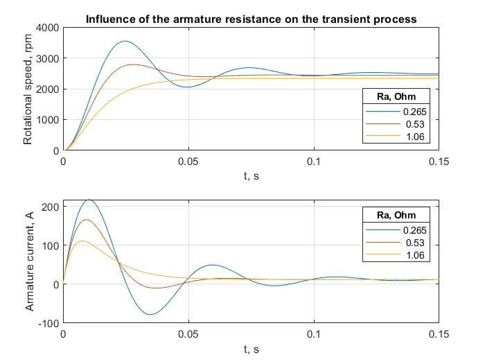
When the resistance of the armature circuit increases, the electromagnetic time constant decreases, the Tem/Ta ratio increases, the number of speed oscillations, the armature current and the electromagnetic moment decreases, the transient becomes aperiodic. In this case, the value of the steady-state rotational speed decreases. Increasing the resistance of the armature winding reduces the value of the starting current, while the value of the steady-state armature current does not change, since it depends on the value of the motor load. The duration of the transient process decreases.
The resistance of the armature can be increased by introducing additional resistance into the armature circuit.
Armature inductance influence
% motor parameters and rated values
Ra = 0.53;                                    % armature winding resistance, Ohm
La = 0.0038;                                  % armature winding inductance, H
J = 0.0051;                                   % armature inertia, kg*m^2
U = 155;                                      % supply voltage, V
Tem = 0.008;                                  % electromechanical time constant, s
Mc = 7;                                       % load torque, N*m
cF = sqrt(Ra*J/Tem);                          % calculation of c*Ф, where c is the back-EMF coefficient and Ф is magnetic flux
Ta = La/Ra;                                   % electromagnetic time constant, s

Lvar=[0.5 1 2]*La;                            % La variation, e.g. 0.5*La or 2*La
figure(6);
for k = 1:length(Lvar)
    La = Lvar(k);
    tspan = [0 0.15];
    w0 = [0 0 0];
    [T, W] = ode45(@(t,w)difsys(t, w, Ra, La, J, Mc, U, cF),tspan,w0);
    W(:,1)=30/pi*W(:,1);
    Mem=W(:,3)*cF;
    hold on;
    subplot(2,1,1);
    plot(T,W(:,1));
    title('Influence of the armature inductance on the transient process');
    xlabel('t, s');
    ylabel('Rotational speed, rpm');
    grid on;

    hold on;
    subplot(2,1,2);
    plot(T,W(:,3));xlabel('t, s'); ylabel('Armature current, A'); grid on;
end
hold off;

subplot(2,1,1); title(legend(num2str(Lvar'),'Location', 'southeast'),'La, H');
subplot(2,1,2); title(legend(num2str(Lvar'),'Location', 'northeast'),'La, H');
As the inductance of the armature increases, the electromagnetic time constant increases, the Tem/Ta ratio decreases, the number of speed oscillations, the armature current and the electromagnetic torque increases, the transient process becomes more oscillatory, but the armature inrush current is decreased at start-up. The steady-state values of armature current and rotational speed do not change. The duration of the transient process increases.
Armature inertia influence
% motor parameters and rated values
Ra = 0.53;                                    % armature winding resistance, Ohm
La = 0.0038;                                  % armature winding inductance, H
J = 0.0051;                                   % armature inertia, kg*m^2
U = 155;                                      % supply voltage, V
Tem = 0.008;                                  % electromechanical time constant, s
Mc = 7;                                       % load torque, N*m
cF = sqrt(Ra*J/Tem);                          % calculation of c*Ф, where c is the back-EMF coefficient and Ф is magnetic flux
Ta = La/Ra;                                   % electromagnetic time constant, s

Jvar=[0.5 1 2]*J;                             % J variation, e.g. 0.5*J or 2*J
figure(7);
for k = 1:length(Jvar)
    J = Jvar(k);
    tspan = [0 0.15];
    w0 = [0 0 0];
    [T, W] = ode45(@(t,w)difsys(t, w, Ra, La, J, Mc, U, cF),tspan,w0);
    W(:,1)=30/pi*W(:,1);
    Mem=W(:,3)*cF;
    hold on;
    subplot(2,1,1);
    plot(T,W(:,1));title('Influence of the armature inertia on the transient process');
    xlabel('t, s'); ylabel('Rotational speed, rpm'); grid on;

    hold on;
    subplot(2,1,2);
    plot(T,W(:,3));xlabel('t, s'); ylabel('Armature current, A'); grid on;
end
hold off;

subplot(2,1,1); title(legend(num2str(Jvar'),'Location', 'southeast'),'J, kg*m^2');
subplot(2,1,2); title(legend(num2str(Jvar'),'Location', 'northeast'),'J, kg*m^2');
Magnetic flux influence (permanent magnets)
% motor parameters and rated values
Ra = 0.53;                                    % armature winding resistance, Ohm
La = 0.0038;                                  % armature winding inductance, H
J = 0.0051;                                   % armature inertia, kg*m^2
U = 155;                                      % supply voltage, V
Tem = 0.008;                                  % electromechanical time constant, s
Mc = 7;                                       % load torque, N*m
cF = sqrt(Ra*J/Tem);                          % calculation of c*Ф, where c is the back-EMF coefficient and Ф is magnetic flux
Ta = La/Ra;                                   % electromagnetic time constant, s

cFvar=[0.8 1 2]*cF;                           % cФ variation, e.g. 0.5*cФ or 1.5*cФ
figure(7);
for k = 1:length(cFvar)
    cF = cFvar(k);
    tspan = [0 0.15];
    w0 = [0 0 0];
    [T, W] = ode45(@(t,w)difsys(t, w, Ra, La, J, Mc, U, cF),tspan,w0);
    W(:,1)=30/pi*W(:,1);
    Mem=W(:,3)*cF;
    hold on;
    subplot(2,1,1);
    plot(T,W(:,1));title('Influence of the excitation flux on the transient process');
    xlabel('t, s'); ylabel('Rotational speed, rpm'); grid on;

    hold on;
    subplot(2,1,2);
    plot(T,W(:,3));xlabel('t, s'); ylabel('Armature current, A'); grid on;
end
hold off;

subplot(2,1,1); title(legend(num2str(cFvar'),'Location', 'southeast'), 'cФ');
subplot(2,1,2); title(legend(num2str(cFvar'),'Location', 'northeast'), 'cФ');
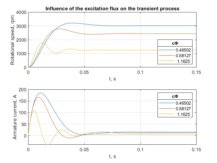
The variation in the magnetic flux significantly affects the steady-state and transient modes of operation of the DC motor. In the steady-state, the amplification of the excitation flux leads to a decrease in the steady-state rotation frequency. The value of the steady-state armature current at a constant load torque decreases, and inrush current during start-up also decreases. The electromechanical time constant sharply decreases, since the excitation flux depends on the degree of minus 2. The ratio of the time constants decreases, the transient process acquires an oscillatory character.
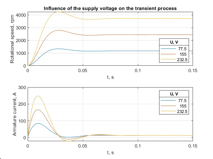
The change in the applied voltage affects the steady-state values of the speed and starting currents. As the applied voltage increases, the speed of rotation increases and the starting currents of the motor increase.
Conclusions
The parameters of DC machine have a significant effect on the type of the transient and on the steady-state values of the armature speed and current.
REFERENCES:
References
- Dr. İsmail H. ALTAŞ, Dynamic Model of a Permanent Magnet DC Motor, Projects for Students, Karadeniz Technical University, Faculty of Engineering, Electrical and Electronics Engineering (URL: http://www.ihaltas.com/courses/fbe_elk5320/eng/projects/Project_37.pdf)
- Manish Mor, Keval Chandarana, Shree Gohil, Sagar Paneliya “Evaluation of the Transient Response of a DC motor International Journal of Advance Engineering and Research” Development (IJAERD), Volume 4,
- Saad, Muhammad, Transient Response of a Separately Excited DC Motor Under No-Load Condition (April 29, 2016). Available at SSRN: https://ssrn.com/abstract=2772630or http://dx.doi.org/10.2139/ssrn.2772630