Project 1 (Mini Project on Vehicle Direction Detection
AIM:
To identify the direction of the vehicle based on the camera input.
General Overview:
Identifying the direction of the vehicle is one of the important & diverse features in Autonomous driving & Advanced Driver Assistance Features. This particular sub-feature of identifying the direction of the vehicle is identifying the direction the vehicle is taking based on the camera input.
The camera reads the road signs & stores them into its memory with unique values for a left turn, right turn & straight drive. Depending on the direction it is taking, the final indication is given to the driver – as an indication if he is driving in the recommended direction or not.
Vehicle Direction Determination can also be coupled alongside features like GPS systems to identify whether the vehicle is reaching its destination in an optimized manner. This sub-feature can also be used along with Lane Detection, Highway Warning, Ramp Entry / Exit in Wrong Way Detection, etc.
The objective of the Mini Project:
- Development of MATLAB Simulink model as per requirement.
- Tag the requirements to the Simulink model; tagging requirements 1 & requirement 2 to their corresponding subsystems is fine.
- MBD compliant changes, Data Dictionary creation & code generation is added advantage, and that is not the scope of this project.
- If choosing code generation, Storage class for Input signals: ImportedExtern; Storage class for Output signal: Export to File; Storage class for local signals: localizable; Storage class for calibration signals: Const.
- Choose sample time for all signals as 0.01s
SOLUTION;
GIVEN
Signals & Calibration Data List:
|
Signal / Calibration Name |
Signal Type |
Data Type |
Dimension |
Min |
Max |
Initial Value |
Units |
|
SteeringWheel_YawDegreeInput |
Input |
Int16 |
1 |
-180 |
180 |
- |
Deg |
|
CameraInput_RoadSign |
Input |
Boolean |
1 |
0 |
1 |
- |
- |
|
Vehicle_Turn_Status |
Local |
Int16 |
1 |
-180 |
180 |
- |
Deg |
|
Right_Turn_AngularLimit |
Calibration |
Int16 |
[1 1] |
-180 |
180 |
30 |
Deg |
|
Left_Turn_AngularLimit |
Calibration |
Int16 |
[1 1] |
-180 |
180 |
-120 |
Deg |
|
Straight_Drive_Steering_Angle |
Calibration |
Int16 |
[1 1] |
-180 |
180 |
0 |
Deg |
|
RightTurn_RoadSign |
Calibration |
Int16 |
[1 1] |
-180 |
180 |
30 |
|
|
LeftTurn_RoadSign |
Calibration |
Int16 |
[1 1] |
-180 |
180 |
-120 |
|
|
Straight_RoadSign |
Calibration |
Int16 |
[1 1] |
-180 |
180 |
0 |
|
|
Vehicle_Direction_Indicator |
Output |
Boolean |
1 |
0 |
1 |
- |
- |
SIMULINK DATA DICTIONARY (SLDD) FILE CREATION:
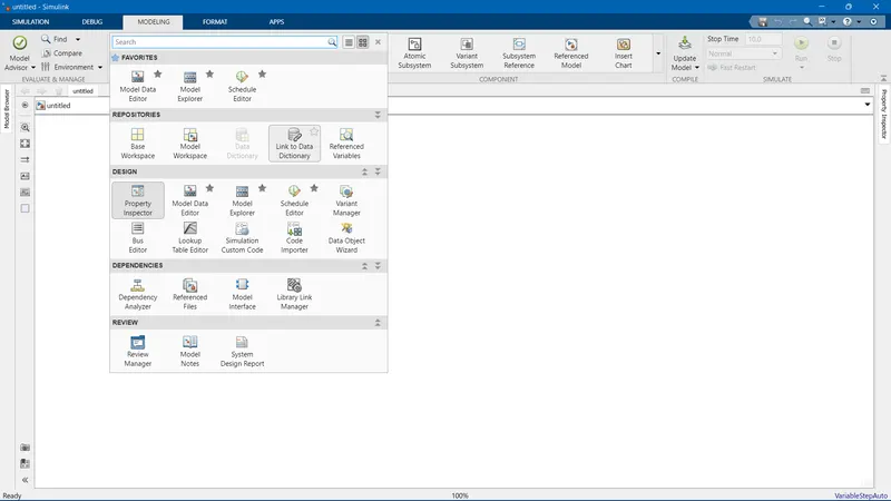
First, we need to create and save the main file on the desktop then, go to modeling>> Link to the Data dictionary
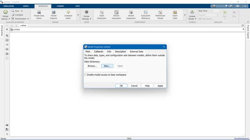
Select New and uncheck Enable model access to the base workspace.
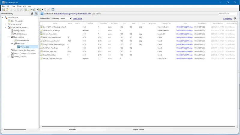
Now the created SLLD file will be below the main file, Expand External Data, and the created SLDD file.
Click on Design Data and start adding all the given input signals and constants with correct datatypes and Right click>> Save changes.
DEVELOPMENT OF THE SIMULINK MODEL:
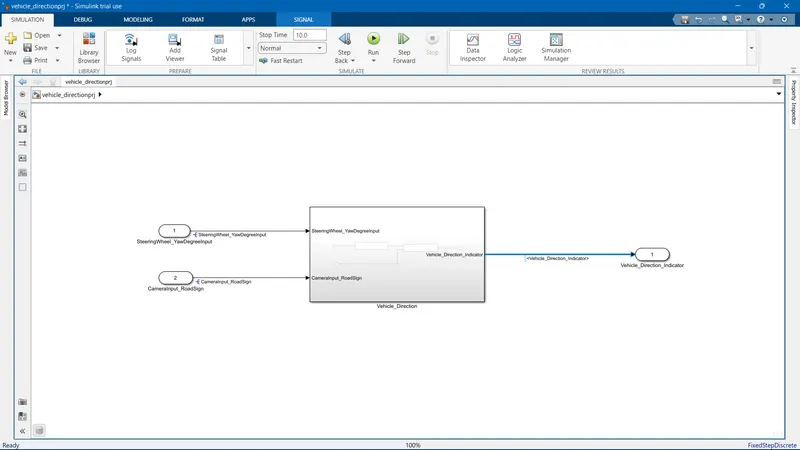
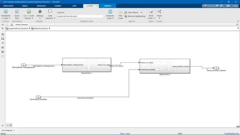
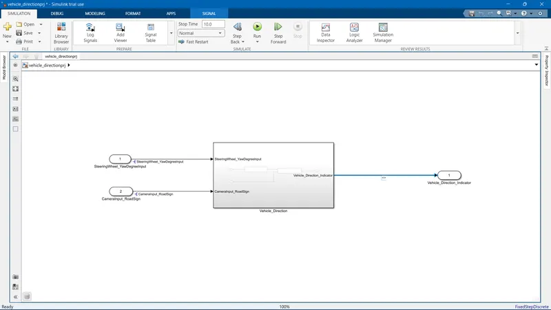
The main subsystem 'Vehicle_Direction' along with inputs 'SteeringWheel_YawDegreeInput', 'CameraInput_RoadSign', and output signal 'Vehicle_Direction_Indicator' is shown below.
The main subsystem 'Vehicle_Direction' is further divided into two more subsystems which are 'Requirement_1' and Requirement_2
Requirement - 1:
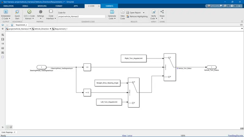
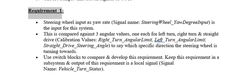
- Steering wheel input as yaw rate (Signal name: SteeringWheel_YawDegreeInput) is the input for this system.
- This is compared against 3 angular values, one each for a left turn, right turn & straight drive (Calibration Values: Right_Turn_AngularLimit, Left_Turn_AngularLimit, Straight_Drive_Steering_Angle) to say which specific direction the steering wheel is turning towards.
- Use switch blocks to compare & develop this requirement. Keep this requirement in a subsystem & the output of this requirement is a local signal (Signal Name: Vehicle_Turn_Status).
Requirement – 2:
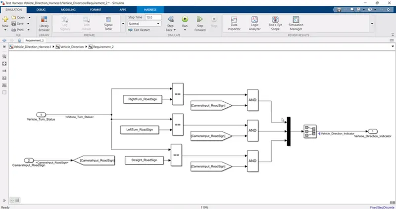
- Keep this requirement as a separate subsystem. Inputs to this requirement are a local signal from requirement 1 (Signal Name: Vehicle_Turn_Status) & an input signal from the camera (Signal Name: CameraInput_RoadSign), which confirms the occurrence of a road sign.
- Signal Vehicle_Turn_Status is compared against calibration values (Calibration Values: RightTurn_RoadSign, LeftTurn_RoadSign, Straight_RoadSign), if each of them is found equal, then each of the three corresponding output is compared against the camera input signal,
- Using a logical operator block, only one among them is finally given as an output signal (Signal Name: Vehicle_Direction_Indicator).
SIGNAL RESOLVING AND PROPAGATING:
Right-click on the signal line which is connected to the inputs and outputs that we wanted to resolve, Right click>> Select properties
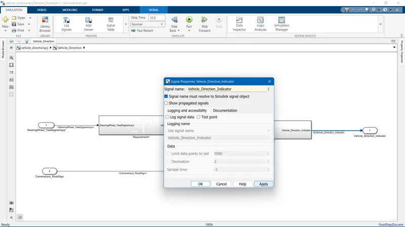
In the signal properties block, Enter the name of the signal also, it needs to be stored in the workspace which corresponds to the signal object.
To propagate the signal, select the signal type corresponding to the similar type and just enter the '<>' symbol and enter.
REQUIREMENTS TAGGING:
We need to open the problem description file [Excel/pdf/Word etc;] in the same path and open it outside the MATLAB and select the particular requirement as shown below,
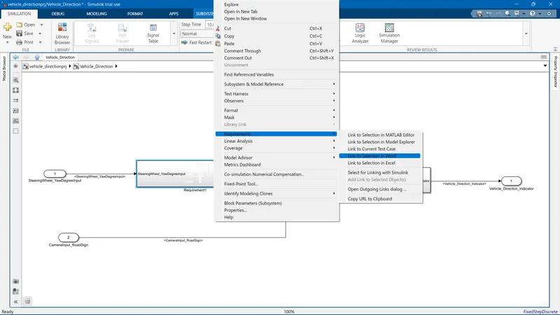
Now, open the model and right-click on the particular requirement (subsystem) where we need to link the excel data to it.
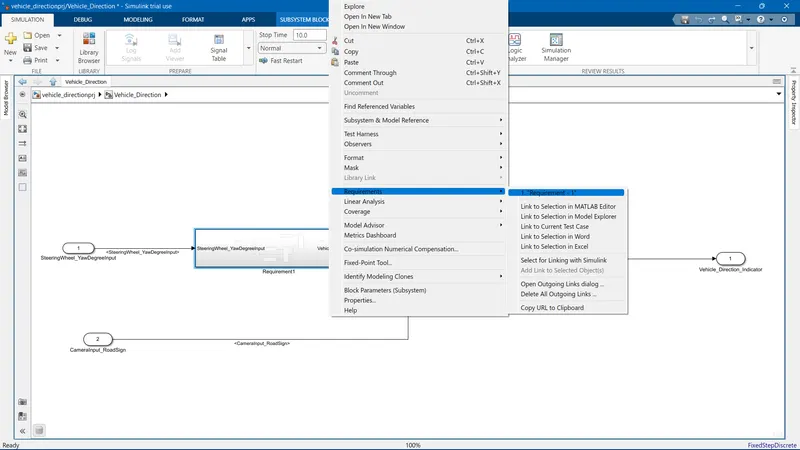
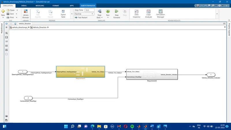
Similarly, it is done for all the requirements in the given problem description.
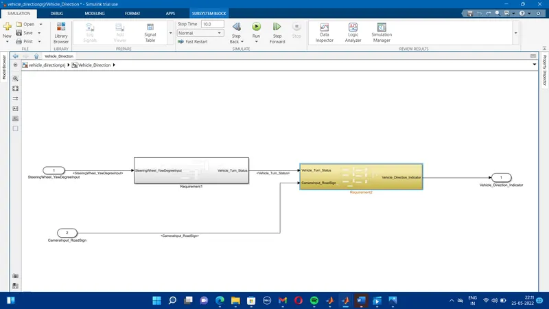
Finally, the model is done with all the requirements tagging, and signal to resolve.
SOLVER SETTING:
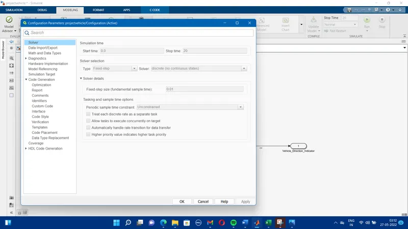
A fixed-step solver with a discrete solver is selected with suitable start/stop and step time.
PRE-CODE SETTING:
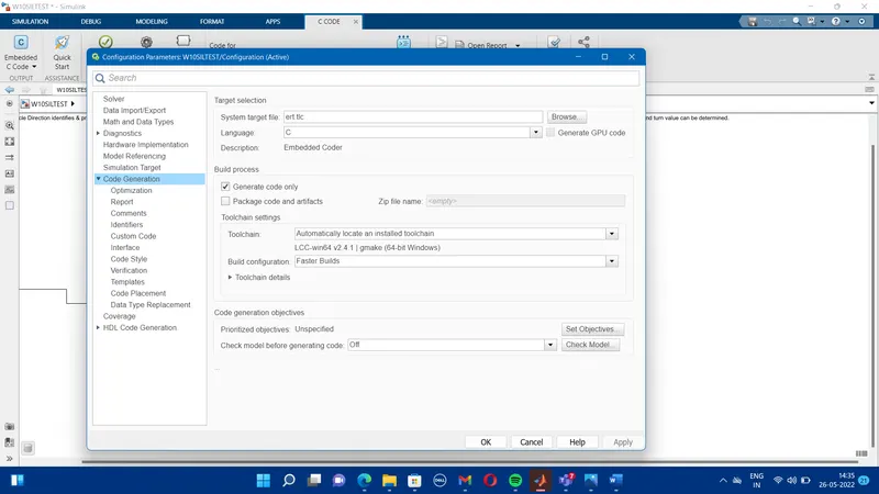
Go to modeling>> select code Generation >> Browse and select Embedded code and apply
MAB GUIDELINES:
Mathworks Advisory Board(MAB) Guidelines are a set of modeling guidelines developed by an independent industry.
To check whether the model which we have developed satisfies and passes the MAB guideless we follow the below steps.
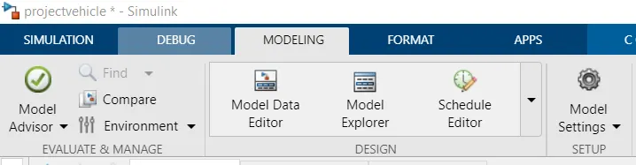
Before the process, we need to simulate our model without error and select the MODEL ADVISOR tab
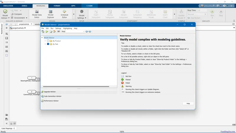
Expand by task and select only Modeling standards by MAB
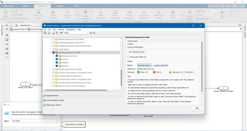
Run the test and click on Generate Report,
Now the generated report will be stored in an HTML file in the current model path which we can access anytime.
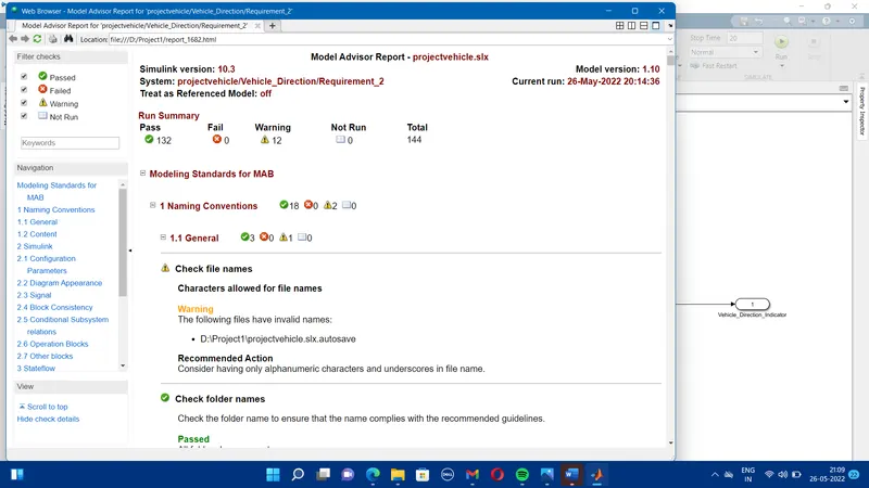
Hence, the model is satisfying the MAB guideless and the test status is PASS.
Now we can generate the code of our model.
THE CODE GENERATION:
The first step of configuring a model for code generation is to choose & configure a code generation target.
When you select a target, other model configuration parameters change automatically.
Parameters such as code interface parameters, build process parameters, and target hardware parameters change automatically.
System Target File (TLC) -ert.tlc Contains pre-configured settings for the code format, target type, coding language, and other software build environment code generation settings.
Model Files:
Model.c Contains the entry point for the algorithm
Model.h Declares the model data structures
Model_private.h Contains local macros & data required by your model
Model_types.h Provides type definitions for user-defined types in the mode.
After SIL test,
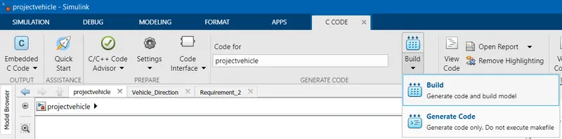
Click on APPS>> BUILD icon from Simulink icons tray.
Code Generation does:
Generates the C-code for the model
Generates MBD traceability files
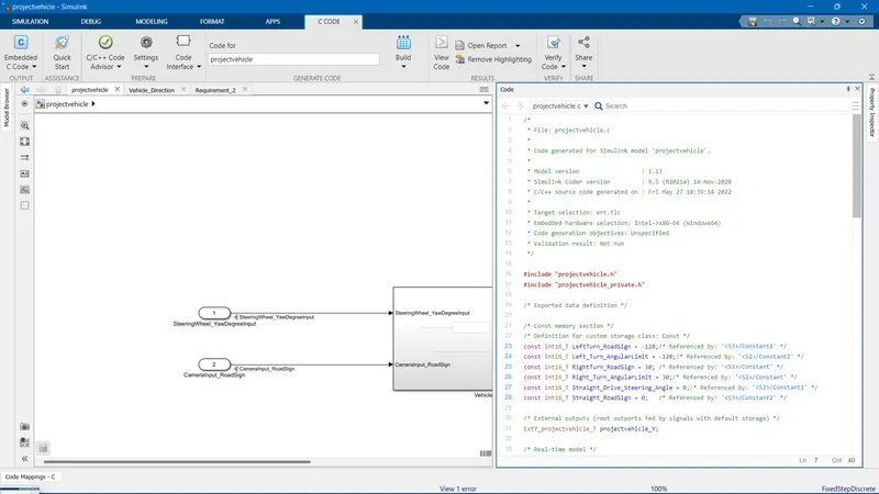
Now we can generate the code of our model.
Go to Apps >> C code >> Embedded code
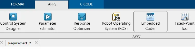
Expand EMbedded coder and select generate code.
1	/*
2	 * File: projectvehicle.c
3	 *
4	 * Code generated for Simulink model 'projectvehicle'.
5	 *
6	 * Model version                  : 1.12
7	 * Simulink Coder version         : 9.5 (R2021a) 14-Nov-2020
8	 * C/C++ source code generated on : Thu May 26 22:58:41 2022
9	 *
10	 * Target selection: ert.tlc
11	 * Embedded hardware selection: Intel->x86-64 (Windows64)
12	 * Code generation objectives: Unspecified
13	 * Validation result: Not run
14	 */
15
16	#include "projectvehicle.h"
17	#include "projectvehicle_private.h"
18
19	/* Exported data definition */
20
21	/* Const memory section */
22	/* Definition for custom storage class: Const */
23	const int16_T LeftTurn_RoadSign = -120;/* Referenced by: '<S3>/Constant1' */
24	const int16_T Left_Turn_AngularLimit = -120;/* Referenced by: '<S2>/Constant2' */
25	const int16_T RightTurn_RoadSign = 30; /* Referenced by: '<S3>/Constant' */
26	const int16_T Right_Turn_AngularLimit = 30;/* Referenced by: '<S2>/Constant' */
27	const int16_T Straight_Drive_Steering_Angle = 0;/* Referenced by: '<S2>/Constant1' */
28	const int16_T Straight_RoadSign = 0;   /* Referenced by: '<S3>/Constant2' */
29
30	/* External outputs (root outports fed by signals with default storage) */
31	ExtY_projectvehicle_T projectvehicle_Y;
32
33	/* Real-time model */
34	static RT_MODEL_projectvehicle_T projectvehicle_M_;
35	RT_MODEL_projectvehicle_T *const projectvehicle_M = &projectvehicle_M_;
36
37	/* Model step function */
38	void projectvehicle_step(void)
39	{
40	  /* local block i/o variables */
41	  int16_T Vehicle_Turn_Status;
42
43	  /* Outputs for Atomic SubSystem: '<Root>/Vehicle_Direction' */
44	  /* Switch: '<S2>/Switch' incorporates:
45	   *  Constant: '<S4>/Constant'
46	   *  Constant: '<S5>/Constant'
47	   *  Inport: '<Root>/SteeringWheel_YawDegreeInput'
48	   *  RelationalOperator: '<S4>/Compare'
49	   *  RelationalOperator: '<S5>/Compare'
50	   *  Switch: '<S2>/Switch1'
51	   */
52	  if (SteeringWheel_YawDegreeInput > 0) {
53	    /* Switch: '<S2>/Switch' incorporates:
54	     *  Constant: '<S2>/Constant'
55	     */
56	    Vehicle_Turn_Status = Right_Turn_AngularLimit;
57	  } else if (SteeringWheel_YawDegreeInput == 0) {
58	    /* Switch: '<S2>/Switch1' incorporates:
59	     *  Constant: '<S2>/Constant1'
60	     *  Switch: '<S2>/Switch'
61	     */
62	    Vehicle_Turn_Status = Straight_Drive_Steering_Angle;
63	  } else {
64	    /* Switch: '<S2>/Switch' incorporates:
65	     *  Constant: '<S2>/Constant2'
66	     *  Switch: '<S2>/Switch1'
67	     */
68	    Vehicle_Turn_Status = Left_Turn_AngularLimit;
69	  }
70
71	  /* End of Switch: '<S2>/Switch' */
72
73	  /* Outport: '<Root>/Vehicle_Direction_Indicator' incorporates:
74	   *  Constant: '<S3>/Constant'
75	   *  Constant: '<S3>/Constant1'
76	   *  Constant: '<S3>/Constant2'
77	   *  Inport: '<Root>/CameraInput_RoadSign'
78	   *  Logic: '<S3>/AND'
79	   *  Logic: '<S3>/AND1'
80	   *  Logic: '<S3>/AND2'
81	   *  RelationalOperator: '<S3>/Relational Operator'
82	   *  RelationalOperator: '<S3>/Relational Operator1'
83	   *  RelationalOperator: '<S3>/Relational Operator2'
84	   */
85	  projectvehicle_Y.Vehicle_Direction_Indicator[0] = (CameraInput_RoadSign &&
86	    (Vehicle_Turn_Status == RightTurn_RoadSign));
87	  projectvehicle_Y.Vehicle_Direction_Indicator[1] = (CameraInput_RoadSign &&
88	    (Vehicle_Turn_Status == LeftTurn_RoadSign));

89	  projectvehicle_Y.Vehicle_Direction_Indicator[2] = (CameraInput_RoadSign &&
90	    (Vehicle_Turn_Status == Straight_RoadSign));
91
92	  /* End of Outputs for SubSystem: '<Root>/Vehicle_Direction' */
93	}
94
95	/* Model initialize function */
96	void projectvehicle_initialize(void)

97	{
98	  /* (no initialization code required) */
99	}
100
101	/* Model terminate function */
102	void projectvehicle_terminate(void)

103	{
104	  /* (no terminate code required) */
105	}
106
107	/*
108	 * File trailer for generated code.
109	 *
110	 * [EOF]
111	 */
112
The code is generated for the modelwhich we have designed and to check the model behavior we are now performing MIL and SIL test.
MODEL IN LOOP (MIL) TESTING:
Model-in-the-loop testing (MIL) and simulation are the techniques used to abstract the behavior of a system or subsystem in a way that the model can be used to test, simulate and verify.
By using an industry-standard toolchain such as Simulink for the model definition we can test and define that model within a desktop environment, allowing a complex system to be managed efficiently.
Once we have modeled your control system or environment (plant model), we can use this plant model to test our controller strategies.
Control strategies are usually tested cases that are developed in tune with the functional requirement of the system.
We have created different Test cases in an Excel sheet and then imported them to the Harness input block
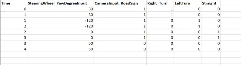
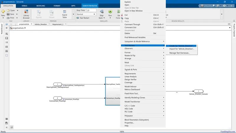
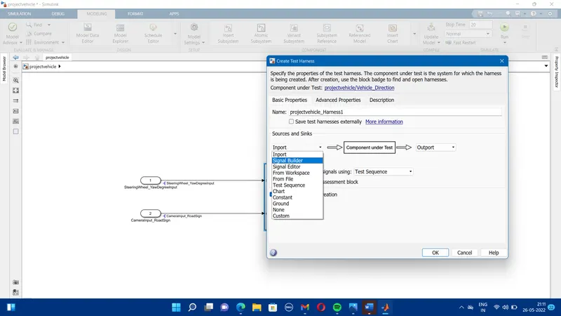
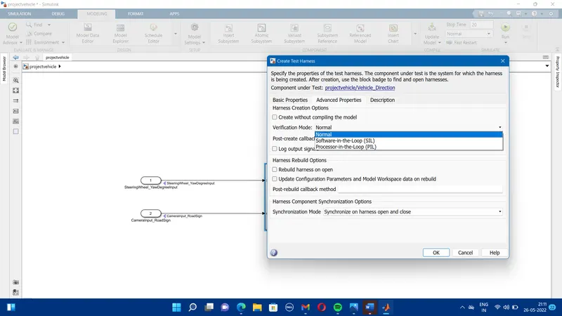
After selecting the MIL test, we get a new harnessed model
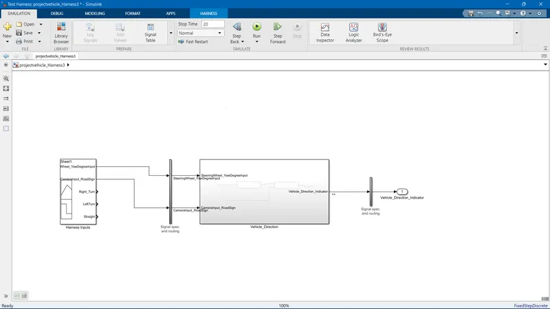
The next step is importing the Test cases to the model by double-clicking on Harness Inputs >> Go to file>> Import from file.
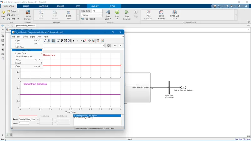
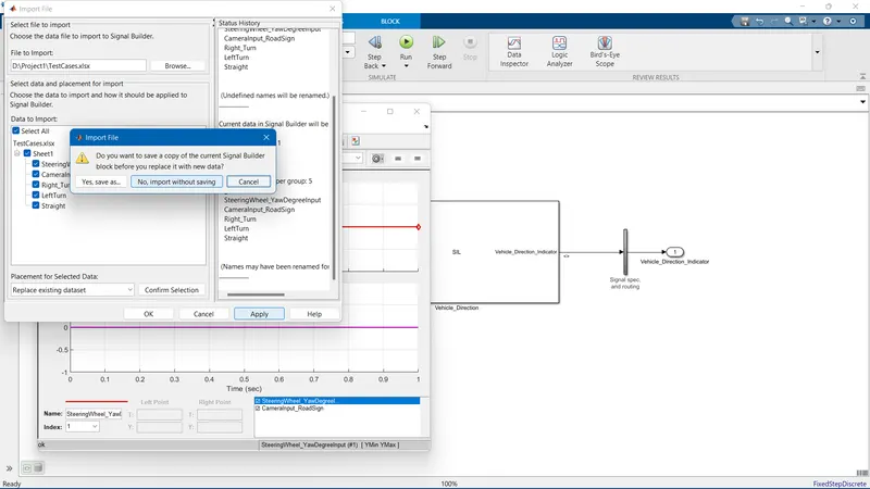
Our test begins by taking the difference between the actual output and the expected output. If the result is zero, then the model which we have created has no error and satisfied the conditions.
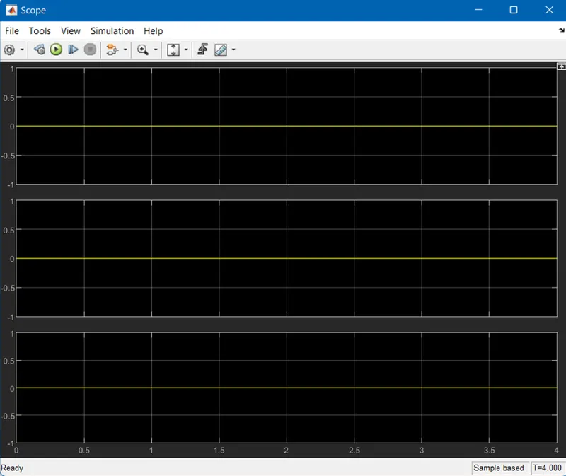
To calculate the difference between the actual output and the expected output, We are considering a sum block with coefficients (+, -) at each output signal and it is plotted in a graph by using the scope block.
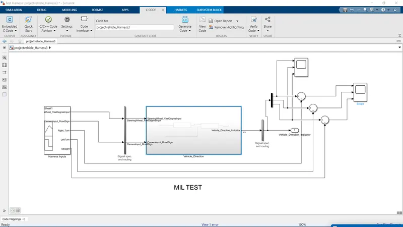
From the below plot it is clear that the difference between the actual output and the expected output is Zero hence the model is said to provide the required output as expected with no errors.
The last optional test is that we can verify whether the actual signal traces the expected signal. i.e, The model has to provide the same output waveform (signal) by tracing the expected signal which is studied below.
Here we are connecting a scope to the output signals and plotting it in a graph and observing it with the input signal.
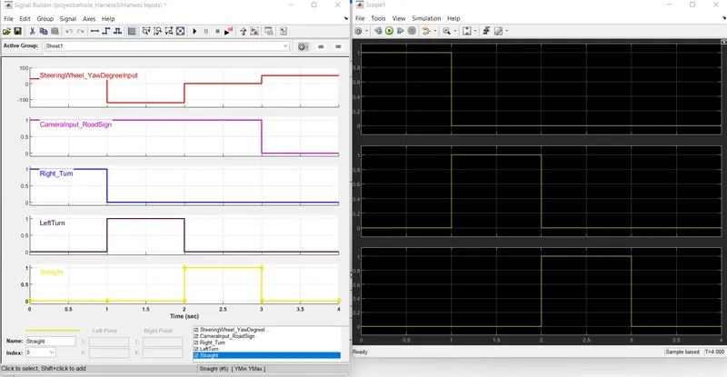
Hence we have completed the MODEL-IN-LOOP TEST for the given model.
SOFTWARE-IN-LOOP (SIL) TESTING :
Software-in-loop testing (SIL) is supported by the MATLAB coder, which enables the user to verify the production-ready source code and compiled object code.
By using an industry-standard tool-chain such as Simulink for the model definition we can test and define that model within a desktop environment, allowing a complex system to be managed efficiently
The template which was exactly used for MIL shall be used for SIL as well. Only replace MATLAB Model block with S Function Builder block before treating the subsystem as atomtic unit.
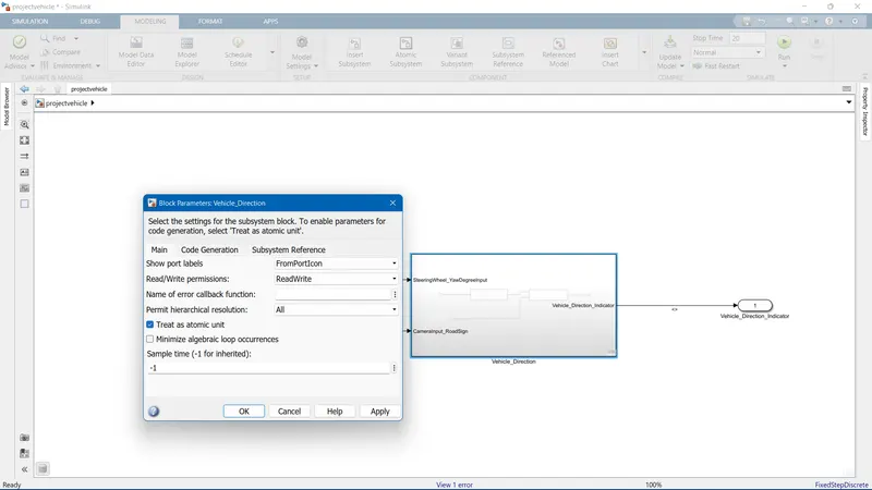
Now selecting the type of input for Test cases as Signal builder and the test type as Soft ware in loop (SIL) as shown below.
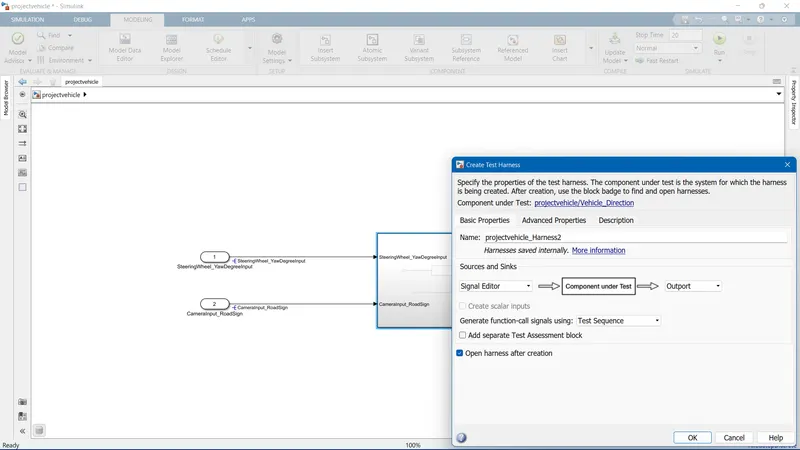
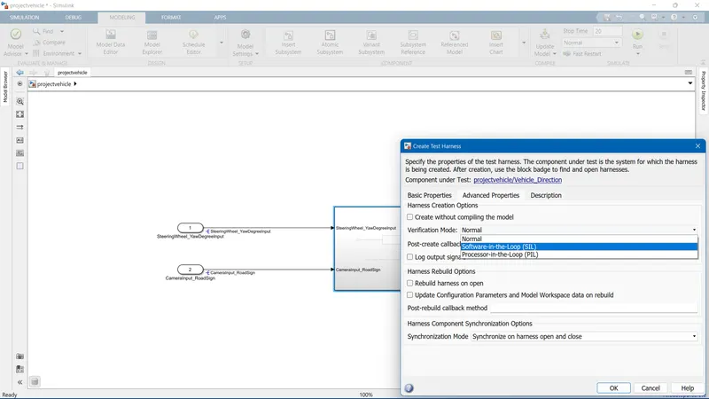
Now the Harnessed model is ready for Testing.
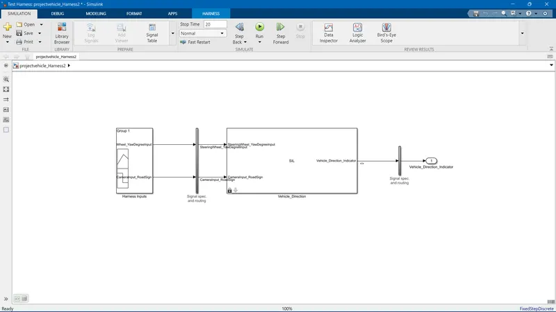
Importing the test case file to the Harness input block as shown below.
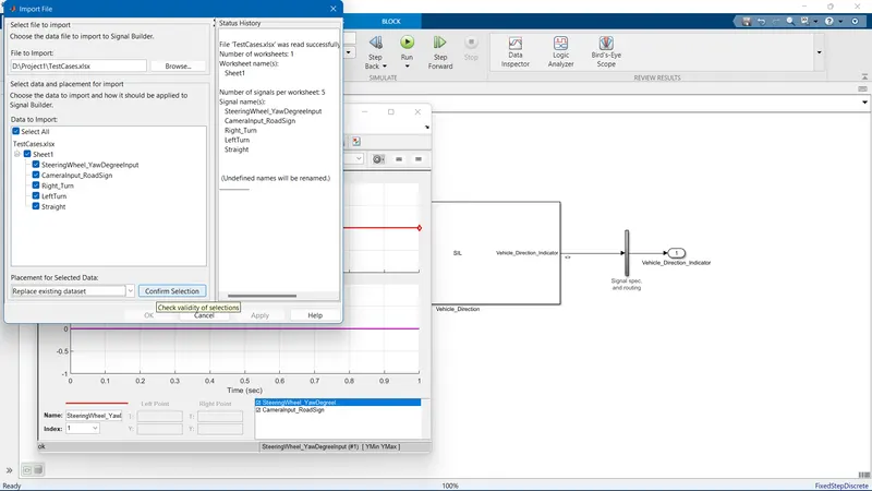
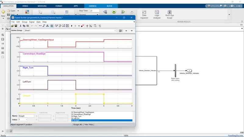
Now the model is ready for Testing with all the necessary Test cases.
Our test begins by taking the difference between the actual output and the expected output. If the result is zero, then the model which we have created has no error and satisfied the conditions.
To calculate the difference between the actual output and the expected output, We are considering a sum block with coefficients (+, -) at each output signal and it is plotted in a graph by using the scope block.
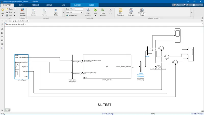
The last optional test is that we can verify whether the actual signal traces the expected signal. i.e, The model has to provide the same output waveform (signal) by tracing the expected signal which is studied below.
Here we are connecting a scope to the output signals and plotting it in a graph and observing it with the input signal.
Hence we have completed the SOFTWARE-IN-LOOP TEST for the given model.