Project 2 - Rankine cycle Simulator
AIM: To create a Rankine cycle simulator using MATLAB:
The Rankine cycle is an idealized thermodynamic cycle describing the process by which certain heat engines, such as steam turbines or reciprocating steam engines, allow mechanical work to be extracted from a fluid as it moves between a heat source and heat sink.
The Rankine cycle is a model used to predict the performance of steam turbine systems. The ability of a Rankine engine to harness energy depends on the relative temperature difference between the heat source and heat sink. The greater the differential, the more mechanical power can be efficiently extracted out of heat energy, as per Carnot's theorem.
The efficiency of the Rankine cycle is limited by the high heat of vaporization of the working fluid. Unless the pressure and temperature reach supercritical levels in the boiler, the temperature range that the cycle can operate over is quite small.
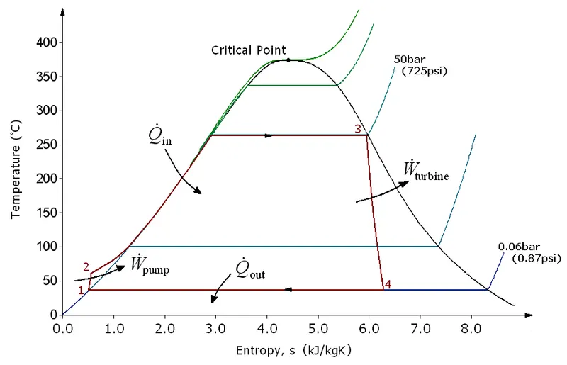
Rankine engines generally operate in a closed-loop where the working fluid is reused. The water vapor with condensed droplets often seen billowing from power stations is created by the cooling systems (not directly from the closed-loop Rankine power cycle). This 'exhaust' heat is represented by the "Qout" flowing out of the lower side of the cycle shown in the T–s diagram below. Cooling towers operate as large heat exchangers by absorbing the latent heat of vapourization of the working fluid and simultaneously evaporating cooling water to the atmosphere.
Rankine cycle consists of an operating fluid that continuously gets evaporated and condensed in a close loop.
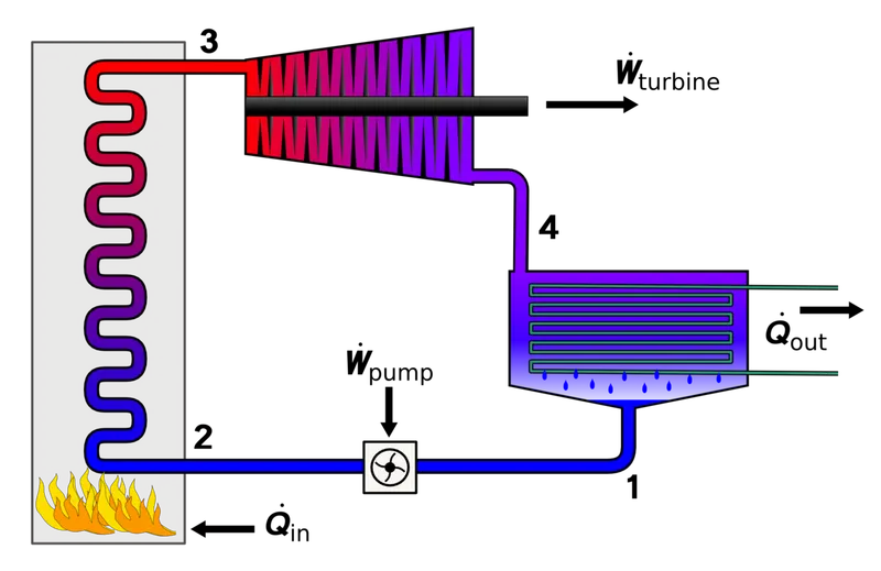
Components used:
1) Boiler for generating steam at constant pressure
2) A turbine or engine in which steam will expand isentropically and work is done
3) A condenser in which heat is removed from the exhaust steam and is completely converted into the water at constant pressure
4) A pump that raises the pressure of liquid water to boiler pressure and pumps it into the boiler for converting into steam.
The Rankine cycle operates in the following steps:
1-2 Isentropic Expansion. The vapor is expanded in the turbine, thus producing work that may be converted to electricity. In practice, the expansion is limited by the temperature of the cooling medium and by the erosion of the turbine blades by liquid entrainment in the vapor stream as the process moves further into the two-phase region. Exit vapor qualities should be greater than 90%.
2-3 Isobaric Heat Rejection. The vapor-liquid mixture leaving the turbine is condensed at low pressure, usually in a surface condenser using cooling water. In well-designed and maintained condensers, the pressure of the vapor is well below atmospheric pressure, approaching the saturation pressure of the operating fluid at the cooling water temperature.
3-4 Isentropic Compression. The pressure of the condensate is raised in the feed pump. Because of the low specific volume of liquids, the pump work is relatively small and often neglected in thermodynamic calculations.
4-1 Isobaric Heat Transfer. High-pressure liquid enters the boiler from the feed pump and is heated to saturation temperature. Further addition of energy causes evaporation of the liquid until it is fully converted to saturated steam.
Governing equations:
In general, the efficiency of a simple Rankine cycle can be written as

Each of the next four equations is derived from the energy and mass balance for a control volume.  defines the thermodynamic efficieny of the cycle as the ratio of net power output to heat input. As the work required by the pump is often around 1% of the turbine work output, it can be simplified.




When dealing with the efficiencies of the turbines and pumps, an adjustment to the work terms must be made:


where;
 |
Heat flow rate to or from the system (energy per unit time) |
 |
Mass flow rate (mass per unit time) |
 |
Mechanical power consumed by or provided to the system (energy per unit time) |
|
Thermodynamic efficiency of the process (net power output per heat input, dimensionless) |
 |
Isentropic efficiency of the compression (feed pump) and expansion (turbine) processes, dimensionless |
 |
The "specific enthalpies" at indicated points on the T-s diagram. |
 |
The final "specific enthalpy" of the fluid if the turbine were isentropic |
 |
The pressures before and after the compression process |
OBJECTIVE:
- Calculating the state points of the Rankine Cycle.
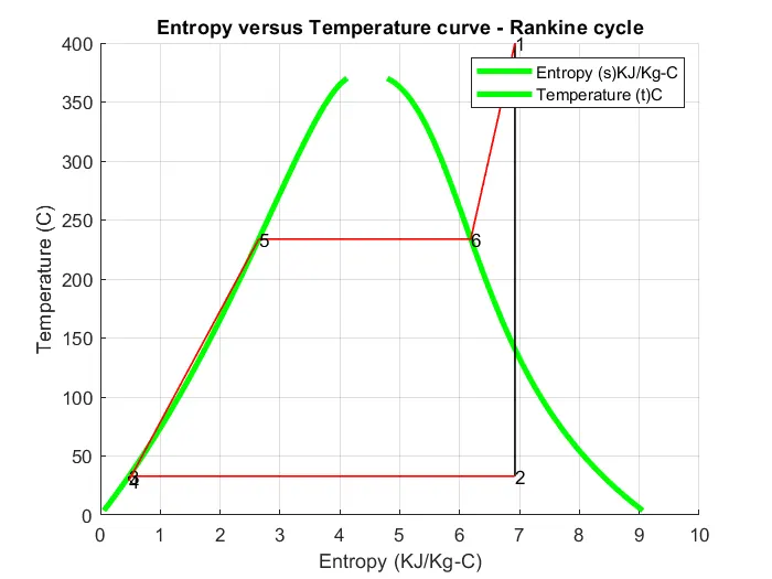
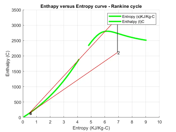
- Plotting T-s and h-s Diagrams for a given set of inputs.
The link for the standard XSteam library to get the steam table data for water is given below. It must be used to calculate the points in between the state variables
"https://drive.google.com/file/d/1RK fvroj3eClaovmltIs3daqHnxkcoU-/view
Now Let us begin our program to simulate the Rankine cycle using MATLAB:
1. MAIN PROGRAM:
%RANKINE CYCLE SIMULATOR
%CALCULATING THE NETWORK OF THE RANKINE CYCLE
%CALCULATING THE BACK WORK RATIO OF THE RANKINE CYCLE
%TAKING VALUES FROM THE USER

clear all
close all
clc

%DISPLAYING THE CONTENT
fprintf("\n                          RANKINE CYCLE SIMULATOR              \n");
fprintf("\nprocess 1-2 : Isentropic expansion in the Turbine\n");
fprintf("\nprocess 2-3 : Isobaric heat rejection by the condensor\n");
fprintf("\nprocess 3-4 : Isentropic compression in the pump\n");
fprintf("\nprocess 4-1 : Isobaric heat addition by the boiler\n");

%REQUESTING THE USER TO GIVE THE INPUTS
p1= input('\n Enter the presuure at the Turnine inlet (in bar) = ');
t1 = input('\n Enter the temperature at the Turnine inlet (in celsius) = ');
p2= input('\n Enter the presuure at the condensor (in bar) = ');

%TURBINE INLET PARAMETERS
tsat_1 = XSteam('Tsat_p',p1);
if t1 > tsat_1
    h1 = XSteam('h_pt',p1,t1);
    s1 = XSteam('s_pt',p1,t1);
elseif t1 == tsat_1
    h1 = XSteam('hV_p',p1);
    s1 = XSteam('sV_p',p1);
else
    fprintf("\n Enter higher value of Turbine inlet temperature (in celsius)!!! nn");
end

%CONDITIONS AT TURBINE OUTLET
%BASED ON THE LOCATION OF POINT 2 THE FOLLOWING VALUES/PROPERTIES ARE
%EVALUATED
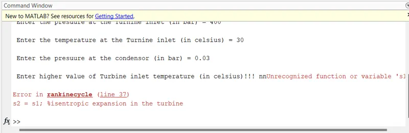
s2 = s1; %isentropic expansion in the turbine
ssat_2 = XSteam('sV_p',p2);
if s2 < ssat_2
    sf_2 = XSteam('sL_p',p2);
    sg_2 = XSteam('sV_p',p2);
    %let x denote the dryness fraction of the steam in the system
    x = (s2 -sf_2)/(sg_2 - sf_2);
    hf_2 = XSteam('hL_p',p2);
    hg_2 = XSteam('hV_p',p2);
    h2 = hf_2 + x*(hg_2 - hf_2);
    t2 = XSteam('Tsat_p',p2);
else
    x = 1;
    h2 = XSteam('hV_p',p2);
    t2 = XSteam('Tsat_p',p2);
end

%CONDITIONS AT PUMP INLET
p3 = p2;
t3 = XSteam('Tsat_p',p3);
h3 = XSteam('hL_p',p3);
s3 = XSteam('sL_p',p3);
v3 = XSteam('vL_p',p3);

%CONDITIONS AT BOILER INLET
p4 = p1;
s4 = s3;
v4 = XSteam('v_ps',p4,s4);
cp4 = XSteam('Cp_ps',p4,s4);
cv4 = XSteam('Cv_ps',p4,s4);
gamma = cp4/cv4;
G = (gamma - 1)/gamma;
t4 = t3*(p2/p1)^G;

%WORK REQUIRED BY PUMP
W_p = v3*(p4 - p3)*100;
%W_p = h4 -h3
h4 = W_p + h3;

%CONDITION OF INTERMEDIATE STATES: STATE 5 AND STATE 6 IN (4-1) STAGE
t5 = XSteam('Tsat_p',p4);
s5 = XSteam('sL_P',p4);
t6 = t5;
s6 = XSteam('sV_p',p4);

%WORKDONE BY THE TURBINE
W_t = h1 -h2;

%HEAT INPUT
Q_in = h1 -h4;

%HEAT OUTPUT
Q_out = h2 -h3;

%NET_WORK OBTAINED
W_net = W_t - W_p;

%Efficiency of the rankine cycle
efficieny = (W_net*100)/Q_in;

%BACK WORK RATIO
BWR = W_p/W_t;

%SPECIFIC STEAM CONSUMPTION
SSC = 3600/W_net;

%DISPLAYING THE OBTAINED INFORMATION
fprintf("\n                          RESULTS              \n");
fprintf("At state point 1:                    At State point 4: \n p1 = %.2f bar                        p4 = %.2f bar \n T1 = %.2f C                         T4 = %.2f C \n H1 = %.2f KJ/Kg                    H4 = %.2f KJ/Kg \n s1 = %.2f KJ/Kg-C                     S4 = %.2f KJ/Kg-C \n",p1,p4,t1,t4,h1,h4,s1,s4);
fprintf("At state point 2:                    At State point 3: \n p2 = %.2f bar                         p3 = %.2f bar \n T2 = %.2f C                          T3 = %.2f C \n H2 = %.2f KJ/Kg                    H3 = %.2f KJ/Kg \n s2 = %.2f KJ/Kg-C                     S3 = %.2f KJ/Kg-C \n",p2,p3,t2,t3,h2,h3,s2,s3);

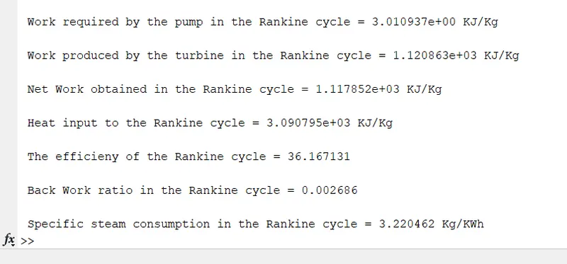
fprintf(" \n Work required by the pump in the Rankine cycle = %d KJ/Kg\n",W_p);
fprintf(" \n Work produced by the turbine in the Rankine cycle = %d KJ/Kg\n",W_t);
fprintf(" \n Net Work obtained in the Rankine cycle = %d KJ/Kg\n",W_net);
fprintf(" \n Heat input to the Rankine cycle = %d KJ/Kg\n",Q_in);
fprintf(" \n The efficieny of the Rankine cycle = %f \n",efficieny);
fprintf(" \n Back Work ratio in the Rankine cycle = %f \n",BWR);
fprintf(" \n Specific steam consumption in the Rankine cycle = %f Kg/KWh \n",SSC);

%PLOTTING THE CURVES

%Plotting Rankine cycle TS Diagram
%Plotting saturation curve
T = linspace(0,373.946,100); %critical point of water at 373.946Degree celsius
figure(1);
hold on
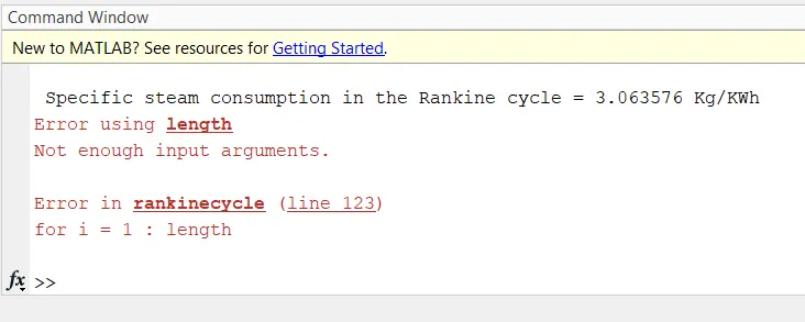
for i = 1 : length(T)
    s_l(i) = XSteam('sL_T',T(i));
    s_g(i) = XSteam('sV_T',T(i));
    h_l(i) = XSteam('hL_T',T(i));
    h_g(i) = XSteam('hV_T',T(i));
end

plot(s_l,T,'linewidth',3,'Color','g');
plot(s_g,T,'linewidth',3,'Color','g');
plot([s1 s2],[t1 t2],'linewidth',1,'Color','k');
text(s1,t1,'1');
plot([s2 s3],[t2 t3],'linewidth',1,'Color','r');
text(s2,t2,'2');
plot([s3 s4],[t3 t4],'linewidth',1,'Color','k');
text(s3,t3,'3');
plot([s4 s5],[t4 t5],'linewidth',1,'Color','r');
text(s4,t4,'4');
plot([s5 s6],[t5 t6],'linewidth',1,'Color','r');
text(s5,t5,'5');
plot([s6 s1],[t6 t1],'linewidth',1,'Color','r');
text(s6,t6,'6');
xlabel('Entropy (KJ/Kg-C)');
ylabel('Temperature (C)');
title('Entropy versus Temperature curve - Rankine cycle');
legend('Entropy (s)KJ/Kg-C','Temperature (t)C');
grid on
hold off

%Plotting Rankine cycle HS Diagram
%Plotting Saturation curve
figure(2);
hold on
plot(s_l,h_l,'linewidth',3,'Color','g');
plot(s_g,h_g,'linewidth',3,'Color','g');
plot([s1 s2],[h1 h2],'linewidth',1,'Color','k');
text(s1,h1,'1');
plot([s2 s3],[h2 h3],'linewidth',1,'Color','r');
text(s2,h2,'2');
plot([s3 s4],[h3 h4],'linewidth',1,'Color','k');
text(s3,h3,'3');
plot([s4 s1],[h4 h1],'linewidth',1,'Color','r');
text(s4,h4,'4');
xlabel('Entropy (KJ/Kg-C)');
ylabel('Enthalpy (C)');
title('Enthapy versus Entropy curve - Rankine cycle');
legend('Entropy (s)KJ/Kg-C','Enthalpy (t)C');
grid on
hold off
CODE EXPLANATION:
- The code begins with the introduction of the Rankine Cycle to the user and mentions the process and its nature.
- The user is then posed with remarks to feed the data. Which takes in the values of p1, t1, and p2. The turbine inlet parameters are defined. Initially, the saturation temperature is found out at pressure p1, by invoking a Matlab defined function i.e, XSteam. If the turbine inlet temperature is higher than the saturation temperature at pressure pl, then, the values of hl and sl are invoked using XSteam at the pressure pl and temperature t1.
- And if the temperature t1 is equal to the saturation temperature then the enthalpy and entropy occur in the vapor region and the values can be invoked by XSteam at the pressure pl. These values are computed using the if and else-if conditions. if the temperature does not satisfy either of these conditions, then another value of turbine inlet temperature is required to run the Rankine Cycle. .it is evident from the process that stages 1 to 2 comprise Isentropic Expansion i.e., s2 = s1, in the Turbine where work is produced.
- On the parallel lines as the temperature if the entropy at state 2 is less than the saturated entropy value at the pressure p2 i.e., s2 < ssat2, then dryness fraction must be considered. The entropy of saturated liquid and saturated vapor is calculated using XSteam at the pressure p2. The value of the dryness fraction is calcuated as follows:
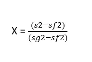
- The value of the enthalpy at state 2 is calculated using the dryness fraction and the values of enthalpy hf and hg which are obtained using XSteam function at the pressure p2.
- The temperature t2 corresponds to the saturation temperature at the pressure of p2. Otherwise, the dryness fraction is 1. Then, the values of enthalpy and temperature ie, h2 corresponds to the enthalpy of the saturated liquid at pressure p2 and t2 is the saturated temperature at pressure p2.
- The above values are computed using if and else conditions. From the Rankine cycle theory, stage 2 to 3 is isobaric heat rejection and therefore, p3 = p2.
The pump inlet conditions are calculated in a very straightforward manner of directly invoking XSteam function at pressure p3. The values of temperature(saturation), specific volume, enthalpy, entropy are calculated. Process 3-4 is Isentropic compression which occurs in the pump. In this, the entropy of states 3 and 4 are equal i.e., s4 and s3. Process 4-1 is an isobar heat addition process that occurs in the steam generator and therefore, the pressure at the state and 4 are the same i.e., p4 = p1.
The specific volume at stage 4 is calculated by using XSteam function with a value to be calculated at pressure p4 and entropy s4. The same values of pressure and entropy are used to evaluate the values of specific heat at constant pressure and volume at state 4 using XSteam function.The adiabatic index is calculated by taking the ratio of specific heat at constant pressure to that at constant volume. By the means of adiabatic gas law, the temperature of state 4 is calculated. The work done by the pump is calculated using the values V3, p4, and p3. Using the work done by the pump, and the known value of h3, the value of enthalpy at state 4 is calculated as mentioned in the Thermodynamic relations section.
The temperature of the process 4-1 intersects the saturated liquid line on the TS curve at 5, where the temperature corresponds to the saturated temperature at p4 and the entropy at state 5 is the entropy of the saturated liquid at p4. The same process 4-1l meets the saturated vapor line at point 6 where the temperature remains the same as that at point 5 i.e., t6 = t5. And the entropy at point 6 corresponds to the entropy of the saturated vapor at p4
The same process 4-1 meets the saturated vapor line at point 6 where the temperature remains the same as that at point 5 ie, t6 = t5. And the entropy at point 6 corresponds to the entropy of the saturated vapor at p4. The values of Work done by the turbine, heat input, heat rejected, net-work, efficiency, back work ratio, and specific steam consumption are calculated as mentioned in the earlier section. To plot the saturation curve in the TS diagram, a numerical array T is assigned and using linspace the values range from 0°C to 373.946°C (critical point of the water) wherein the range is divided into 100 equal parts. The saturated values to be plotted on figure (1) origin from a for loop, where a for loop is run along the length of the numerical temperature array T on the values of entropy and enthalpy at saturated liquid and saturated vapor phases. While plotting the saturation curve on the TS curve, the values of entropy from the for loop are quoted along with the temperature array separately for saturated liquid and saturated vapor. The linewidth is maintained at 3 and is colored in green
A legend is written along with labeling the axes. The plot is titled "Temperature versus Entropy Curve Rankine Cycle.".Similarly, the HS curve is plotted. While plotting the saturation curve on the HS curve, the values of enthalpy from the for loop are quoted along with the temperature array separately for saturated liquid and saturated vapor. The linewidth is maintained at 3 and is colored in cyan The other points are plotted as mentioned below: A legend is written along with Labeling the axes, The plot is titled "Enthalpy versus Entropy Curve - Rankine Cycle." The values of the pressure, temperature, enthalpy, and entropy are calculated for each state and printed in the command window along with the thermodynamic properties.
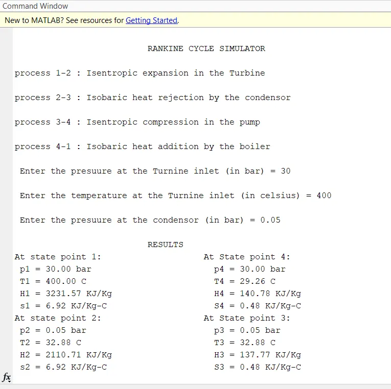
OUTPUT RESULT IN COMMAND WINDOW:
PLOTING OF T-s and H-s Diagram for the given input:
ERRORS WHILE PROGRAMMING:
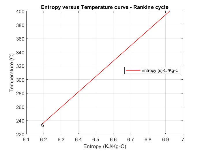
1. Error without using hold on command:
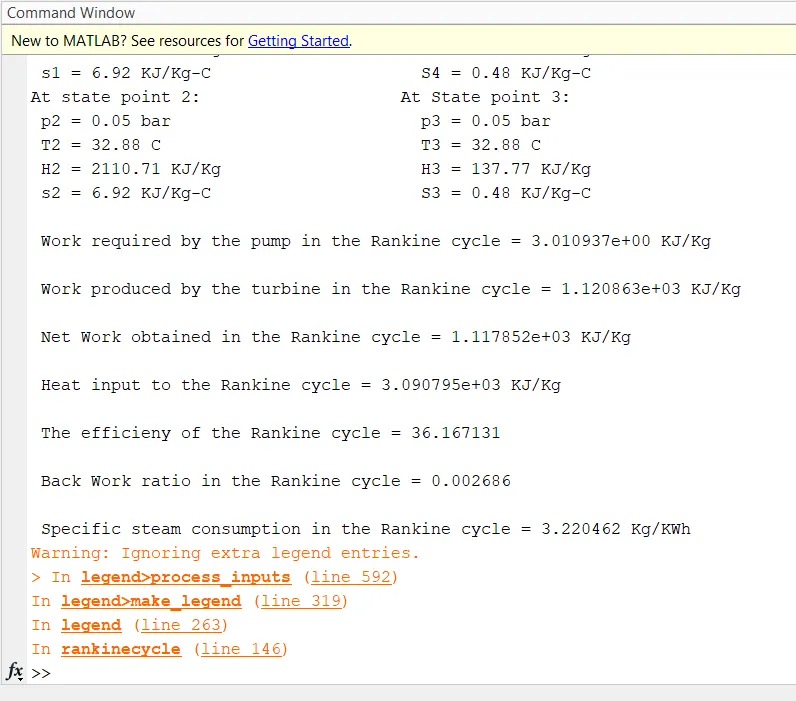
2. Error due to unspecified length of temperature range:
3. Error due to missing of the address variable:

4. Error due to varying the length of linspace command range:
CONCLUSION:
The Rankine Cycle Simulator has been established with required inputs fed. The required variables have been calculated and respective plots have been set up. It is possible to modify the Rankine Cycle by adding desired equipment based on our preference of functionality.
REFERENCES: