Final Project: Design of an Electric Vehicle
**This project is based on the guidelines provided by the trainer for the 13th batch live session. Please consider while grading**
Aim:
To design a system-level configuration electric vehicle.
Theory:- An electric vehicle (EV) is an automotive vehicle that uses one or more electric motors for propulsion. It can be powered by a collector system, with electricity from extravehicular sources, or it can be powered autonomously by a battery (sometimes charged by solar panels, or by converting fuel to electricity using fuel cells or a generator) EVs include, but are not limited to, road and rail vehicles, surface and underwater vessels, electric aircraft and electric spacecraft.
Components of an EV:
EVs do not need the fuel engine and gear transmission, the two of the most crucial components for internal combustion vehicles.
An electric-powered car has three primary components Battery, a motor controller, and the electric motor
- Battery: The battery of an electric car can be charged through the use of ordinary grid electricity at a specialized power station. But aside from the conventional lithium-ion battery technologies, other major battery technologies can be used for electric cars
- Lithium-lon Batteries: This battery technology gives extra performance and range. However, it also carries the highest price tag. Lithium-ion batteries are lighter than Lead-acid and Nickel-metal. These are also the batteries used in digital cameras and smartphones.
Lead Acid Batteries: This battery technology is the most popular. It is also the cheapest among the battery technologies. What's good about it is it’s 97% recyclable.
Nickel Metal Hydride Batteries: This battery technology provides a higher output and better performance but it costs much more than lead-acid batteries.
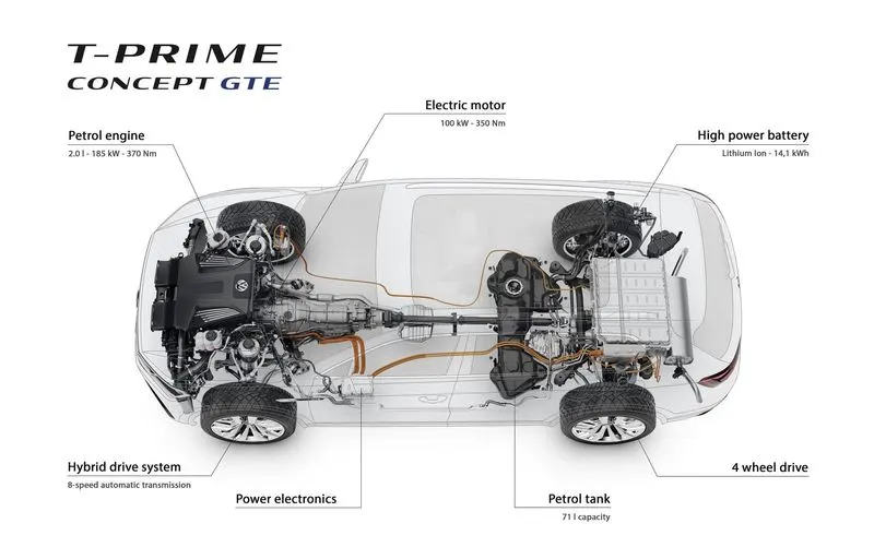
- Motor Controller: The motor controller of an electric car administers its complete operation and the distribution of its power at any given moment. It acts as a floodgate between the motor and batteries. It helps monitor and regulates alt key performance indications such as the vehicle s operator, moto, battery, and accelerator pedal. It has a microprocessor that can limit or redirect current. It is used to either improve the mechanical performance of the car or cut the operator's driving style. There are also more refined controls that are capable of greater accuracy.
PROCEDURE:
In Matlab for EV modeling, it contains a drive cycle block where we provide a specific drive cycle which is a graph plotted between Velocity on the y-axis and time on the x-axis.
Then this data is transmitted to a driver controller unit which contains a person sitting inside the car waiting for the commands from the data which we entered. According to the information, this system accelerates the vehicle, and decelerates or brakes the vehicle. The actual velocity is given as feedback to this system. The power converter contains an H-Bridge Dc power converter to control the motor parameters, we don’t want to connect the battery terminals directly connected to the motor. Here we also provide regenerative braking. A battery system is connected to the power converter which fuels the vehicle.AS the vehicle run that is accelerating the battery discharges and when braking or decelerating the battery gets charged by regenerative braking. The State Of Charge (SOC) can be analyzed. Here for traction purposes, we are using a Permanent Magnet DC motor It drives the transmission system and l powers the wheels. And all this system is situated in the vehicle body In this vehicle body block, we can enter the conditions of the vehicle, grade ability, and wind velocity. and it also contains the transmission system and tires as well. In the tire section, we can enter the tire conditions like a slip, rolling resistance, etc.
Specifications of designing Matlab Electric car (Assumed)
Kerb weight = 750 kg
Frontal area = 0.6m2
Tire rolling radius = 0.3m
Gear ratio = 5
Rear wheel drive 50kW,48V
permanent magnet DC motor .80V,50Ah battery
VEHICLE MODEL:
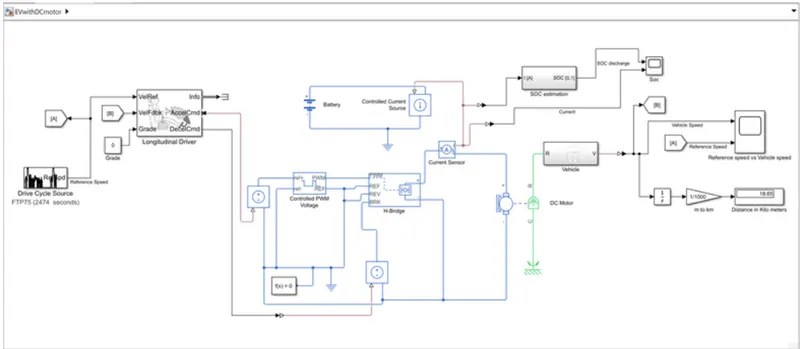
Model Link:
Vehicle body:
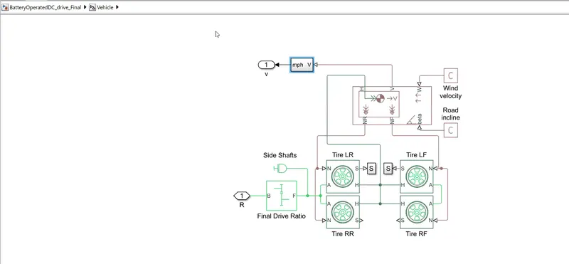
Represents a two-axle vehicle body in longitudinal motion. The block accounts for body mass, aerodynamic drag, road incline, and weight distribution between axles due to acceleration and road profile. The vehicle can have the same or a different number of wheels on each axle.
Optionally include pitch and suspension dynamics or additional variable mass and inertia. The vehicle does not move vertically relative to the ground. Connection H is the mechanical translational conserving port associated with the horizontal motion of the vehicle body.
The resulting traction motion developed by tires should be connected to this port. Connections V, NF, and NR are physical signal output ports for vehicle velocity and front and rear normal wheel forces, respectively. Wheel forces are considered positive if acting downwards.
Connections W and beta are physical signal input ports corresponding to headwind speed and road inclination angle, respectively. If the variable mass is modeled, the physical signal input ports CG and M are exposed. CG accepts a two-element vector representing the x and y distance offsets from vehicle CG to additional load mass CG. M represents the additional mass.
If both variable mass and pitch dynamics are included the physical signal port J accepts the inertia of the additional mass about its CG. The velocity of the vehicle is taken out from the V port of the vehicle’s body. Gradeability is given through the Beta port and it is connected to PS constant block where we can change the values Wind velocity can be given through the W port and it is also connected to PS constant block.
Tyre (Magic formula):
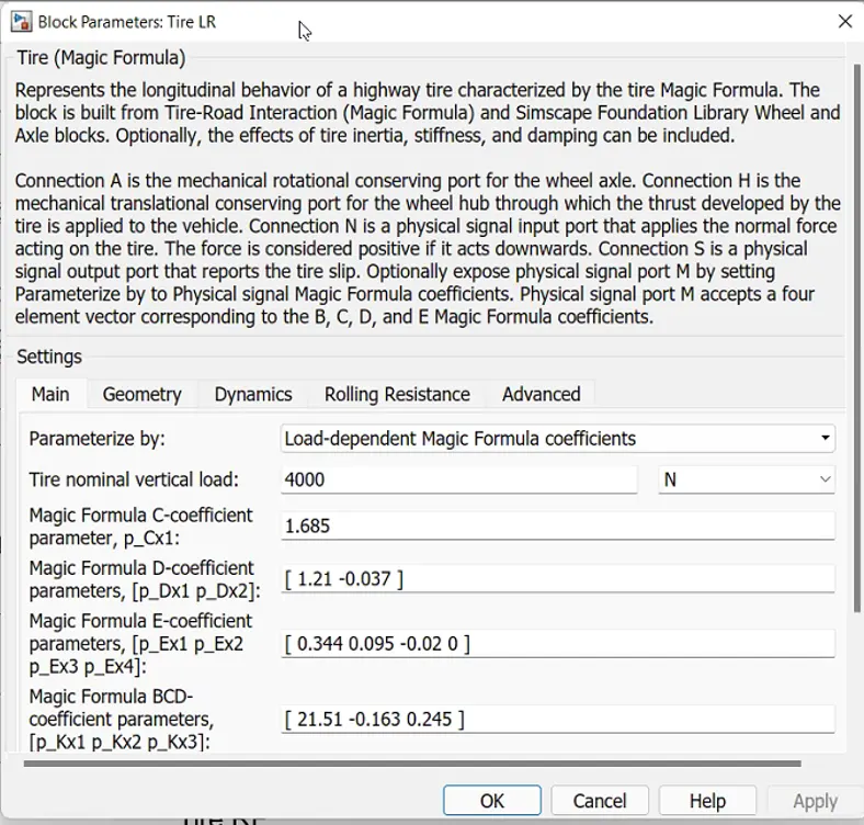
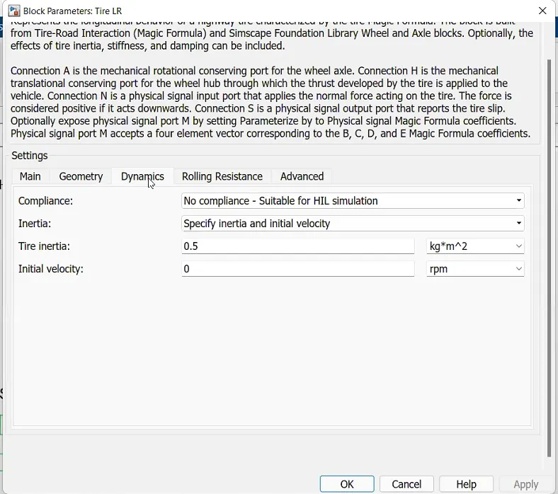
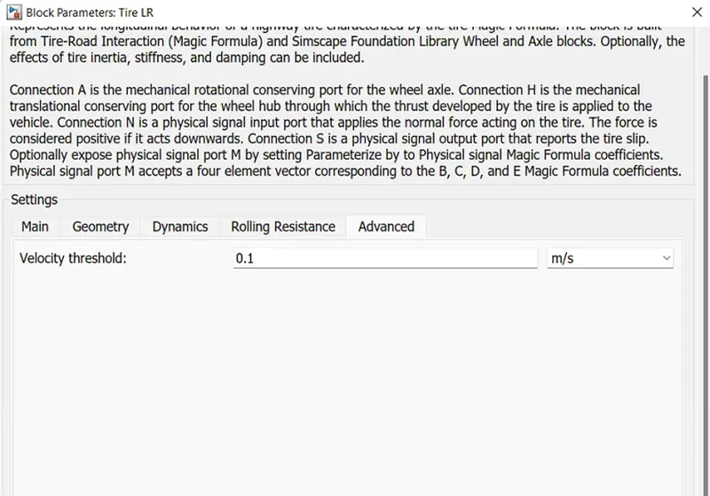
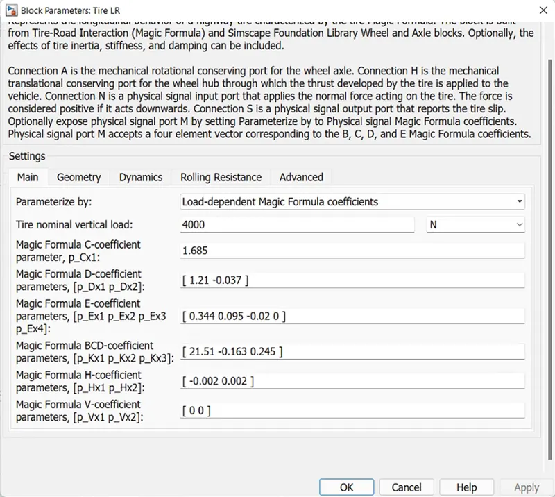
It Represents the longitudinal behavior of a highway tire characterized by the tire Magic Formula. The block is built from Tire-Road Interaction (Magic Formula) and Simscape Foundation Library Wheel and Axle blocks. Optionally, the effects of tire inertia, stiffness, and damping can be included. Connection A is the mechanical rotational conserving port for the wheel axle. Connection H is the mechanical translational conserving port for the wheel hub through which the thrust developed by the tire is applied to the vehicle. Connection N is a physical signal input port that applies the normal force acting on the tire.
The force is considered positive if it acts downwards. Connection S is a physical signal output port that reports the tire slip. Optionally expose physical signal port M by setting Parameterize by to Physical signal Magic Formula coefficients. Physical signal port M accepts a four-element vector corresponding to the B, C, D, and E Magic Formula coefficients.
We have connected all the hub parts of all 4 tires to the hub of the vehicle body. Rear tires and Front tires are specified in the image Normal force acting on the Tire is given through port N and for rear tires, N is connected to the NR of the vehicle body and for Front tires, the 'N is connected to the NF of the electric vehicle body. Here we are not giving any slip to the tires. The slip is given through the Sport. And it is terminated with a terminator block. The Axle of the front tires is connected Axle of the rear tires is connected to the simple gearbox since it is a rear-wheel-drive Here we are not giving any rolling resistance
Permanent Magnet DC motor:
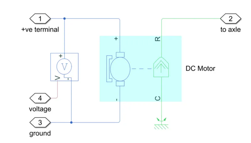
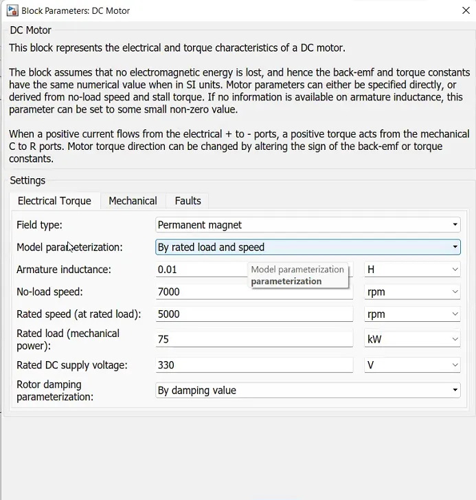
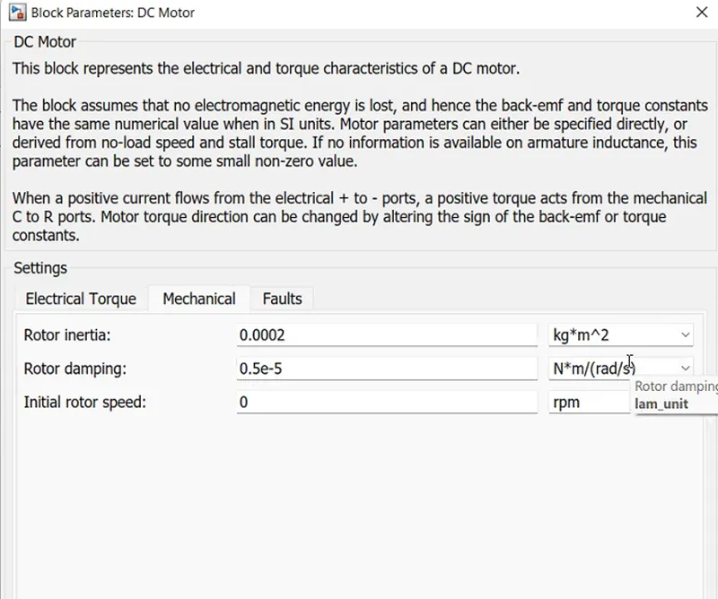
This block represents the electrical and torque characteristics of a DC motor The block assumes that no electromagnetic energy is lost, and hence the back-emf and torque constants have the same numerical value when in St units. Motor parameters can either be specified directly or derived from the no-load speed and stall torque. if no information is available on armature inductance, this parameter can be set to some small non-zero value. When a positive current flows from the electrical + to - ports, a positive torque acts from the mechanical C to Reports. Motor torque direction can be changed by altering the sign of the back emf or torque constants.
The armature of the motor is shown in blue color. The armature is given a voltage that is the output of the H Bridge This Voltage is measured using a voltmeter connected parallel to the motor. The motor rated mechanical power is 50kw The motor rated voltage is 48V DC supply No-load speed is selected as 5000rpm At rated load, the speed is 3000rpm The C port is the casing where it is connected to the mechanical rotational reference The R port is the Rotary part it is connected to the simple gear transmission. The selected values are specified below,
H-Bridge:
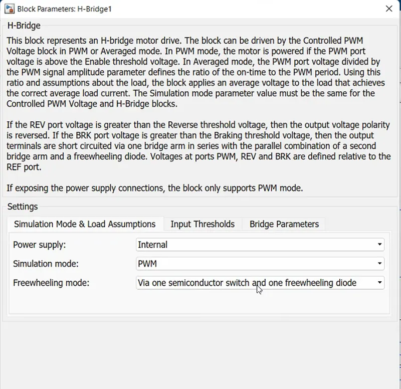
This block represents an H-bridge motor drive. The block can be driven by the Controlled PWM Voltage block in PWM or Averaged mode. In PWM mode, the motor is powered if the PWM port voltage is above the Enable threshold voltage. In Averaged mode, the PWM port voltage divided by the PWM signal amplitude parameter defines the ratio of the on-time to the PWM period.
Using this ratio and assumptions about the load, the block applies an average voltage to the load that achieves the correct average load current.
The Simulation mode parameter value must be the same for the Controlled PWM Voltage and H-Bridge blocks. If the REV port voltage is greater than the Reverse threshold voltage, then the output voltage polarity is reversed.
If the BRK port voltage is greater than the Braking threshold voltage, then the output terminals are short-circuited via one bridge arm in series with the parallel combination of a second bridge arm and a freewheeling diode. Voltages at ports PWM, REV, and BRK are defined relative to the REF Sportif exposing the power supply connections, the block only supports PWM mode.
The regenerative braking option is enabled The simulation time is averaged otherwise simulation takes more time The output voltage amplitude is 300V The specified values are given below.
longitudinal driver:
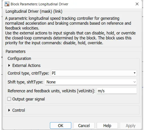
A parametric longitudinal speed tracking controller for generating normalized acceleration and braking commands based on reference and feedback velocities. Use the external actions to input signals that can disable, hold, or override the closed-loop commands determined by the block. The block uses this priority for the input commands: disable, hold, override. The longitudinal driver simply gives acceleration and deceleration commands according to the drive cycle data
The velocity data extracted from the drive cycle is given here as a velocity referrer M
The velocity from the vehicle body is taken and it is feedback to this block.
The gain of 3.6 is nothing but converting velocity in m/s to km/hr. Here we can give the gradeability as well through a constant block.
According to the drive cycle, the driver gives the acceleration and deceleration command to the power converter block.
Battery system:
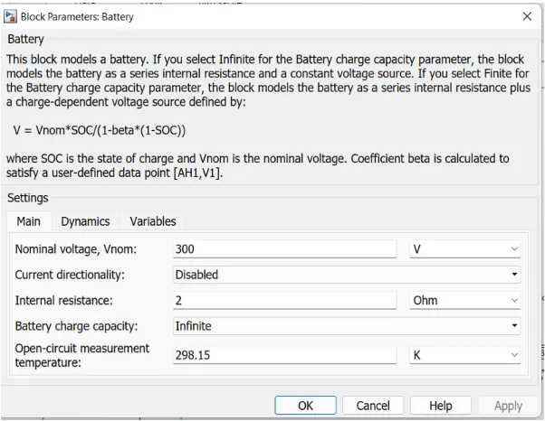
It contains a battery having a nominal voltage of 80V, a controlled current sourceommeterrate transition block, gain blocks, discrete-time integrator, and subtract block.
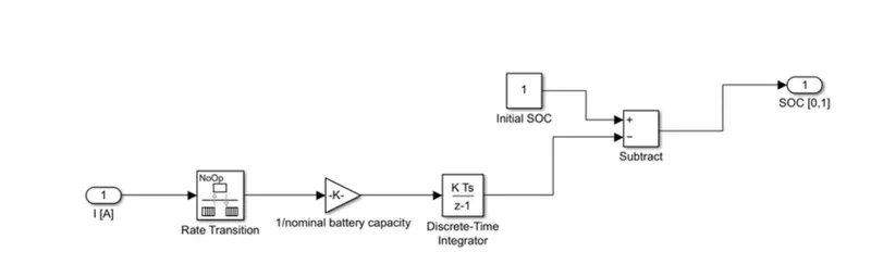
SOC estimation
The soc estimation subsystem is shown below. The discharged SOC is subtracted from the initial SOC to get the Real-time SOC.
Results and Observations:
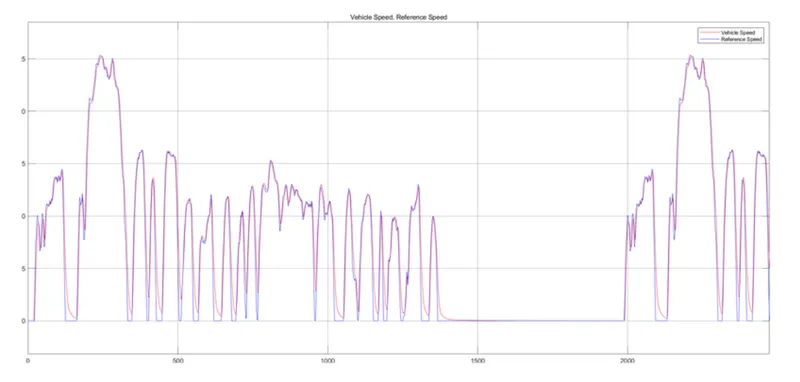
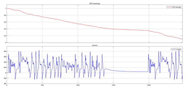
The simulation is done for 2474 seconds as FTP 75 cycle time is 2474 seconds. The results are obtained as follows.
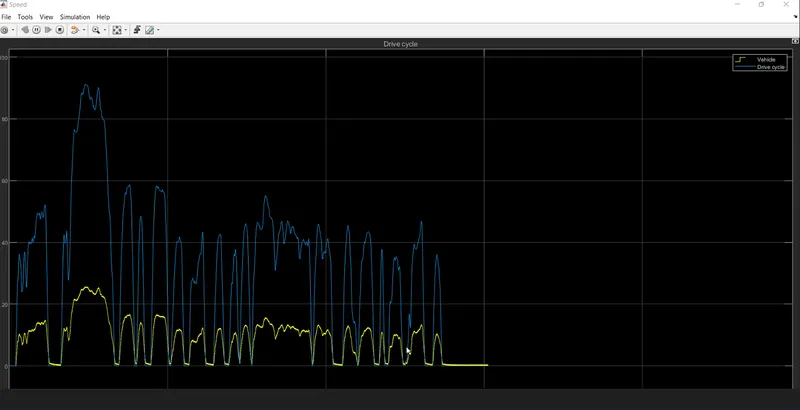
From the above results, the vehicle traced the given Drive cycle and the car traveled a distance of 18.65 km which is nearly the same as the FTP distance of 17.76 km.