Week 3 - Solving second order ODEs
Program to simulate the motion of the pendulum:
In engineering, ODE is used to describe the transient behaviour of a system. A simple example is a pendulum.
The way the pendulum moves depends on the Newtons second law of motion which can be written in the form of ordinary differential equation. But here we get a second order differential equation that describes the position of the ball wrt time.
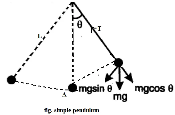
A simple pendulum consists of a point mass ‘m’ hanging on a string of length ‘L’. It is then pulled up to some initial angles θ radians and allowed to oscillate freely under the influence of gravity. At the extreme and end points, the angular velocity is zero and angular displacement is maximum. Whereas, at the exactly vertically downwards point the displacement is zero and angular velocity is maximum. Due to frictional effect the oscillations slowly die down which is controlled by the damping co-efficient (b).
The motion of the pendulum is governed by the following equation:
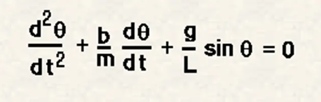
Our objective is to write a program that solves the above ODE. This ODE represents the equation of motion of a simple pendulum with damping.
In the above equation,
g = gravity in m/s2,
L = length of the pendulum in m,
m = mass of the ball in kg,
b=damping coefficient.
To write a program in MATLAB that will simulate the pendulum motion, let us consider:
L = 1metre
m = 1kg
b = 0.05
g = 9.81m/s2
Motion time between = 0-20sec
Angular displacement = 0, angular velocity = 3rad/sec at time =0.
In MATLAB, ODE’s can be solved by 7 solvers. Based on the stiffness they are classified as stiff or non stiff solvers.
In this project, we are going to use ‘ode45’ which is a general-purpose ODE solver but ode45() solves only the 1st order ODE while the simple pendulum damping motion is a 2nd order ODE. So, we need to convert the 2nd order to 1st order by using two variables.
Let us assume that θ1 is θ, which is essentially angular displacement and the derivative of θ1 wrt time is θ2 which is essentially the angular velocity and further the derivative of θ2 wrt time is the angular acceleration.
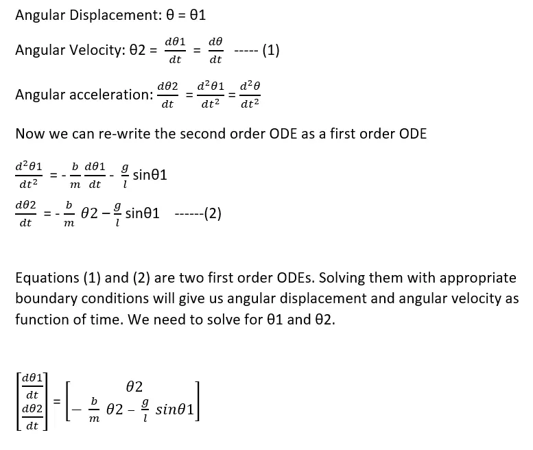
Using this equation, we will define a function to pass it to ode45() function as an argument.
After solving the ODE, we will get an array as output and it has two columns namely; time and result i.e; output = [time, result]
Further the result will have 2 more columns, namely the angular displacement and the angular velocity. i.e; result = [angular displacement, angular velocity]
Using these two values we can get the angular acceleration at any time from the equation.
Now, we are going to use ‘ode45’ which is a general purpose ODE solver.
Ode45 syntax:
[tSol, ySol] = ode45(@(t,y) fName(t,y), [t0, tEnd], y0);
Where;
tSol and ySol are Solution vectors. MATLAB returns ySol for each time tSol
fName is the function that returns dy = F(t.y)
t0 and y0 are the initial conditions representing y(t0) = y0
tEnd is the final value until which the solution is desired.
We are now defining a function which is later called by the main function to solve the ODE.
funcion[dtheta1_dt] = ode_func[t,theta,b,g,l,m]

theta1 = theta(1)
theta2 = theta(2)
dtheta1_dt = theta2;
dtheta2_dt = -(b/m)*theta2-(g/L)*sin(theta1);
dtheta_dt = [dtheta1_dt ; dtheta2_dt];
end
Code explanation:
We are writing a code for the function which is labelled as ‘ode_func’ with the input parameters such as time (t), angle (θ), damping co-efficient (b), acceleration due to gravity (g), length of the string (l) and mass of the bob (m) and then the values are assigned to a variable
‘dtheta_dt’ which is the output variable for the function. So to define this function, first we need to define the output variable which is the function definition.
theta1 and theta2 are the variables that are used to store the two values of input theta.
dtheta1_dt and dtheta2_dt are the variables that store the final simplified form of the equation in the form of matrix so that the function can be called , each parameter can be separated and the simulation can be done easily. dtheta_dt’ is used to store the values in a matrix form. The end command is used to close the function.
Now, we are writing a code for the main program which is used to simulate the motion of the simple pendulum.
Case:1
Once the ODE is solved by the solver and we make a plot, we get the relation between the angular velocity and angular displacement through the below plot.
clear all
close all
clc

b = 0.05;
g = 9.81;
l = 1;
m = 0.1;

%Initial condition
theta_0 = [0;5];

%time points
t_span = linspace(0,20,500);

%solve ode
[t, results] = ode45(@(t,theta) ode_func(t, theta, b,g,l,m),t_span, theta_0);

plot(t,results(:,1))
hold on
plot(t,results(:,2))
ylabel('plot')
xlabel('time')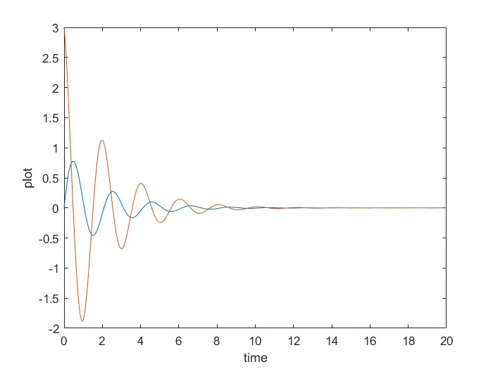
From the below plot, angular velocity is represented in a red line and angular displacement is represented in a blue line.
As per the input data, b, g, l, m are damping co-efficient, gravitational acceleration, length of the pendulum, mass of the pendulum bob respectively;
Plot function is used to plot the required parameters, axis function is used to set the axis of a plot to user-defined x and y axis.
X label and y label is used to label the x-axis and y-axis respectively;
To simulate the motion of the simple pendulum in the graphic format we are now altering the main program as follows:
clear all
close all
clc

b=0.05;
g=9.81;
l=1;
m=1;

%Initial condition
theta_0 = [0;3];

%time points
t_span = linspace(0,20,1000);

%solve ODE
[t, results] = ode45(@(t,theta) ode_func(t, theta, b,g,l,m),t_span, theta_0)

%Plotting
figure(1)
plot(t,results(:,1))
hold on
plot(t, results(:,2))
grid on
axis([0 20 -5 5])
xlabel('time')
ylabel('plot')
legend('displacement','velocity')
title('plot(displacement and angular velocity) vs Time')

%Animation
ct = 1;

for i = 1:length(t)
    x0 = 0;
    y0 = 0;

    x1 = 1*sin(results(i,1));
    y1 = -1*cos(results(i,1));

    figure(2)
    plot([-1 1],[0 0],'linewidth',5,'color','k')
    line([x0 x1],[y0 y1],'linewidth',2,'color','k')
    hold on
    plot(x1,y1,'marker','o','markersize',30,'markerfaceColor','r','markeredgecolor','k')
    title('Transient Motion of a simple Damped pendulum')
    hold off
    axis([-1.5 1.5 -2 0.5])
    pause(0.002)

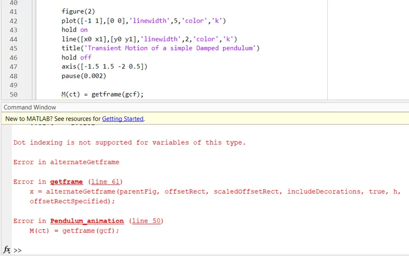
    M(ct) = getframe(gcf);
    ct=ct+1;

end

movie(M)
videofile = VideoWriter('Pendulum_animation.avi','Uncompressed AVI');
open(videofile)
writeVideo(videofile,M)
close(videofile)
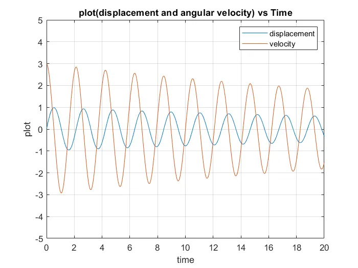
The initial conditions of the angular displacement and angular velocity for time 0 sec is given as 0rad and 3rad/sec. For plotting, figure function is used to assign figure number to that plot. Hold on function is used to plot previous plot. if not used it will plot only the recent plot.
Plot function is used to plot the required parameters, axis function is used to set the axis of a plot to user-defined x and y axis.
X label and y label is used to label the x-axis and y-axis respectively; title function is used to give title to the plot. Ct=1 is taken as initial value for counter to frame.
For each value of angular displacement, we need to repeat the calculation of the co-ordinates and plotting. Hence, to do that we have used For loop.
i=1:length (t)
here i ranges from 1 to the number of values of the time span which in this case is 200
Initially we assign the time interval and divide it in to 200 parts and also enter the initial condition of angular displacement and angular velocity at time t =0.
Next we will define a function and solve the pair of first order ODEs using ode45 function. Then we will plot the angular displacement and angular velocity plots with time and after which we will open the main program which is used to determine the motion of the pendulum by using for loop.
In each iteration of for loop for a particular value of ‘i’ we will use the angular displacement value at that index and locate the position of the bob of pendulum using sin and -cos of that angle.
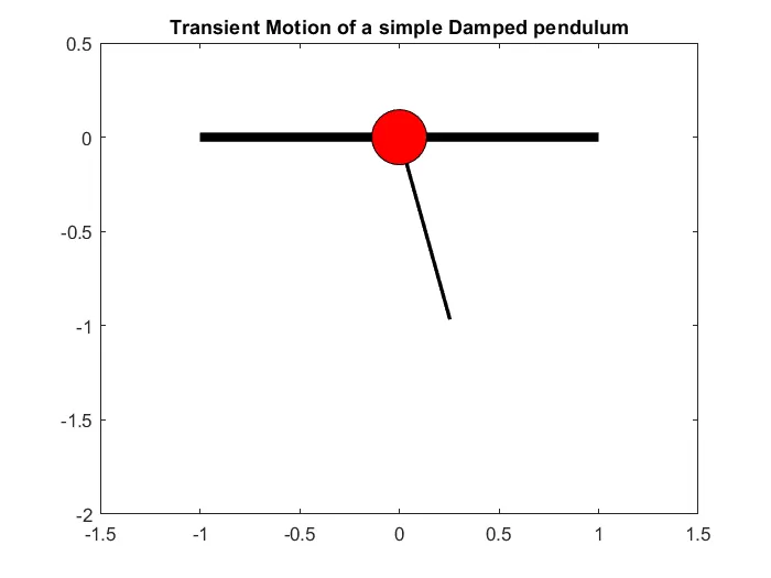
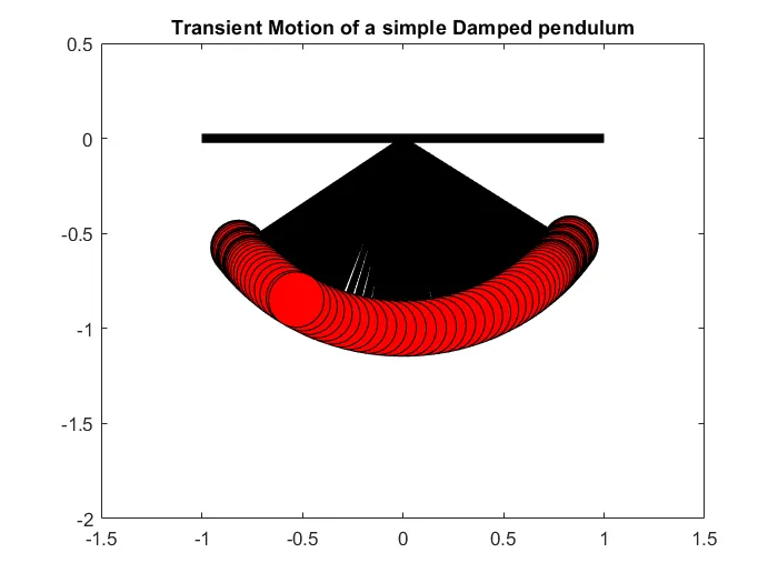
Here in the below plot it is evident that two lines have been plotted to show the ceiling and rod of pendulum and hold value is kept on so that these lines do not disappear. A red circle (‘o’) has been drawn to show the location of the bob. At the end of the for loop, the hold value is changed to off so the current image of the pendulum is removed and a new one can be plotted.
A pause interval of 0.005sec has been introduced so that we can see the fig.
To define the axis of the pendulum; we take the start of the pendulum rod as x0 = 0, y0 = 0 and the end of the pendulum rod is taken as
x1 = l*sin(angular_displacement)
y1 = -l*cos(angular_displacement)
The pendulum bob is plotted using x1 and y1 co=ordinates using o marker having marker size of 25.
M(ct) = getframe(gcf) – here M is used to save each and every frame which is ct and getframe(gcf) in which gcf represents get current frame. When the plot is made, it appears in a figure. So getframe is used to get the particular figure and it saves in the form of an array called ‘M’.
Ct=ct+1 is used to increment the value of the frame to get the next frame.
movie(M) is used because MATLAB is going to generate a movie from all those frames.
Videowriter is used to create a particular video format file.
Open command is used to open up that video file.
Writevideo writes all the frames captured in M in a videofile.
Close -is used to close the video.
output plot:
The graphics/video of the motion of the simple pendulum is provided through a youtube link;
REFER THE BELOW FINAL OUTPUT:
Errors while programming:
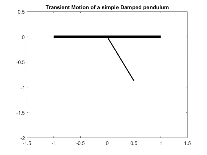
1. Without marker command:
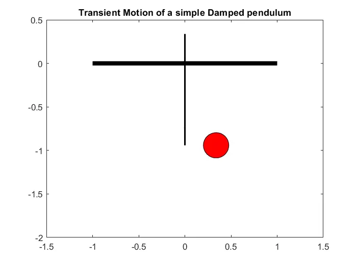
2. Using of hold on commands at various instances:
Errors in command window:
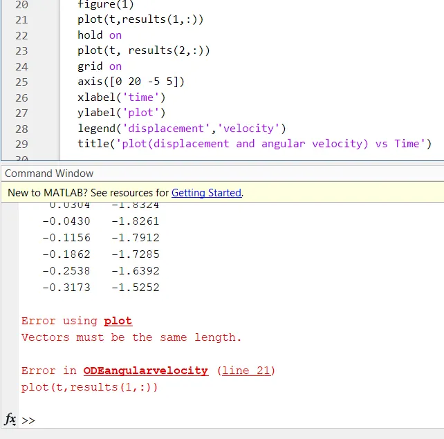
1. For changing the axis of the plots:
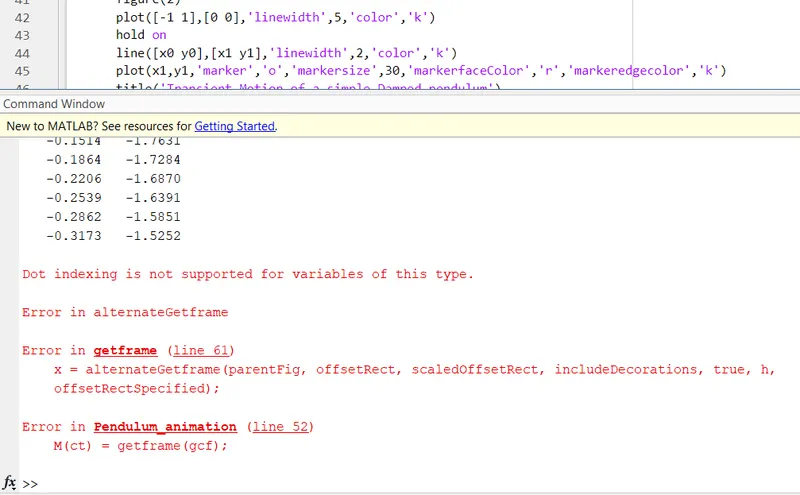
2. Error due to changing the axis of the line command:
3. Error due to changing the axis of the marker command
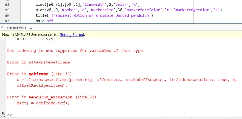
4. Error without marker command: