Week 4.1 - Genetic Algorithm
AIM: To write a code in MATLAB to optimize the stalagmite function and find the global maxima of the function
Genetic Algorithm (GA):
GA is a search-based optimization technique based on the principles of Genetics and Natural Selection. It is frequently used to find optimal or near-optimal solutions to difficult problems. It is used to solve optimization problems, in research, and in machine learning.
Optimization: Optimization is the process of making something better in any process. So, we have a set of inputs and a set of outputs.
Inputs----->|Process|----->Outputs
It refers to finding the values of the inputs in such a way that we get the 'best output values. the 'best refers to maximizing or minimizing one or more objective functions, by varying the input parameter
Stalagmite Function
A stalagmite function refers to the function with which we are generating values over a stalagmite kind of surface for finding out the global maxima and minima local of that particularly given function.
For this, in MATLAB we use a method called 'Optimization. Its criterion is programming which does a selection for the best element with regard to some set of population. Optimization is done by systematically choosing input values from within an allowed set and computing the results of the function. In MATLAB to perform optimization, we use the GA method which is an inbuilt function in MATLAB to find the global maxima of that given stalagmite function.
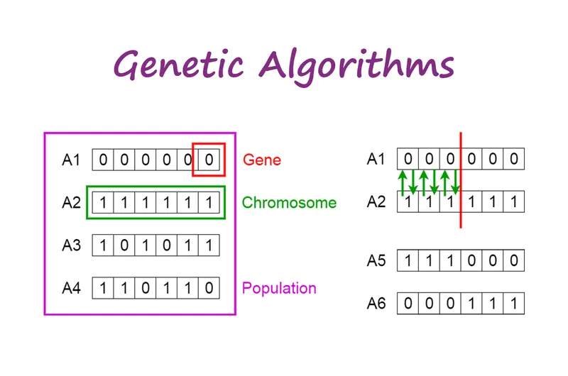
What Are Genetic Algorithms?
A genetic algorithm is a search heuristic that is inspired by Charles Darwin’s theory of natural evolution. This algorithm reflects the process of natural selection where the fittest individuals are selected for reproduction in order to produce offspring of the next generation.
The syntax for this ga() command is as follows
x = ga(fun, nvars) finds a local unconstrained minimum, x, to the objective function,
fun,nvars is the dimension design variables of function.
x= ga(fun,nvars,A,b,Aeq.beq.lb.ub) defines a set of lower and upper bounds on the design variables 'x' so that a solution is found in the range lb ≤ x ≤ ub.
What Are Genetic Algorithms?
A genetic algorithm is a search heuristic that is inspired by Charles Darwin’s theory of natural evolution. This algorithm reflects the process of natural selection where the fittest individuals are selected for reproduction in order to produce offspring of the next generation.
The syntax for this ga() command is as follows
x = ga(fun, nvars) finds a local unconstrained minimum, x, to the objective function,
fun. nvars is the dimension design variables) of function.
x= ga(fun,nvars,A,b,Aeq.beq.lb.ub) defines a set of lower and upper bounds on the design variables, x, so that a solution is found in the range lb ≤ x ≤ ub.
equalities exist for Set A=[]and b=[] and
Set Aeq =[] and beq =[] if no linear equalities exist.
[x, fval] =ga(__) for any previous input arguments, also returns fval, the value of the fitness function at x.
The Notion of Natural Selection: The process of natural selection starts with the selection of the fittest individuals from a population. They produce offspring which inherit the characteristics of the parents and will be added to the next generation. If parents have better fitness, their offspring will be better than parents and have a better chance at surviving. This process keeps on iterating and in the end, a generation with the fittest individuals will be found.
This notion can be applied to a search problem. We consider a set of solutions for a problem and select the set of best ones out of them.
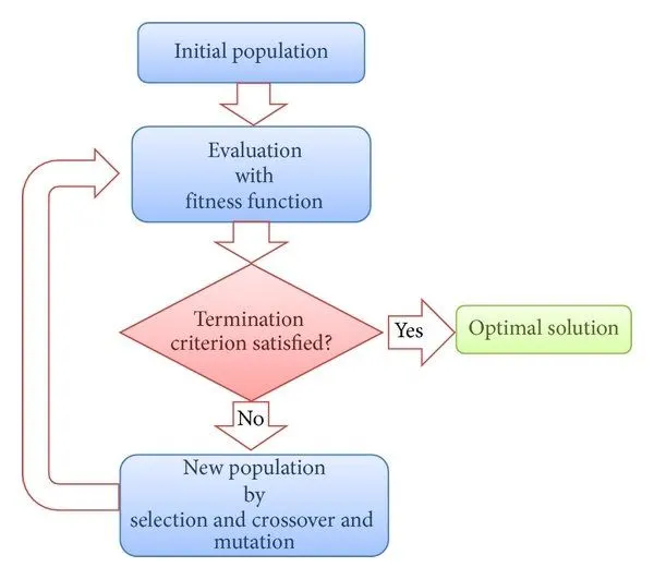
Five phases are considered in a genetic algorithm.
- Initial population
- Fitness function
- Selection
- Crossover
- Mutation
1. Initial Population: The process begins with a set of individuals which is called a Population. Each individual is a solution to the problem you want to solve.
An individual is characterized by a set of parameters (variables) known as Genes. Genes are joined into a string to form a Chromosome(solution)
In a genetic algorithm, the set of genes of an individual is represented using a string, in terms of an alphabet. Usually, binary values are used (strings of 1s and Os). We say that we encode the genes in a chromosome.
2. Fitness Function: The fitness function determines how to fit an individual is (the ability of an individual to compete with other individuals). It gives a fitness score to each individual. The probability that an individual will be selected for reproduction is based on its fitness score.
3. Selection: The idea of the selection phase is to select the fittest individuals and let them pass their genes to the next generation.
Two pairs of individuals (parents) are selected based on their fitness scores. Individuals with high fitness have more chances to be selected for reproduction.
4. Crossover: Crossover is the most significant phase in a genetic algorithm. For each pair of parents to be mated, a crossover point is chosen at random from within the genes.
Offspring are created by exchanging the genes of parents among themselves until the crossover point is reached. The new offspring are added to the population.
5. Mutation: In certain new offspring formed, some of their genes can be subjected to a mutation with a low random probability. This implies that some of the bits in the bit string can be flipped.
Mutation occurs to maintain diversity within the population and prevent premature convergence.
Termination: The algorithm terminates if the population has converged (does not produce offspring which are significantly different from the previous generation). Then it is said that the genetic algorithm has provided a set of solutions to our problem.
The population has a fixed size. As new generations are formed, individuals with the least fitness die, providing space for new offspring
The sequence of phases is repeated to produce individuals in each new generation who are better than the previous generation.
The syntax for Genetic generation Algorithm:
X = ga (fun, nvars)
X =ga (fun, nvars,A, b)
X=ga (fun,nvars,A,b,Aeq, beq)
X =_ga (fun,nvars,A,b,Aeq, beq,1b, ub).
X = ga (fun, nvars,A,b,Aeq, beq,lb,ub,non1con)
X= ga (fun,nvars,A, b,Aeq, beq,lb,ub, non1con,options)
X = ga (fun, nvars, A, b, [], [], 1b, ub, non1con, IntCon)
X = ga (fun, nvars, A, b, [], [], 1b, ub, non1con, IntCon, options)
X=ga(problem)
[x,fval] = ga(___)[x,fval. exitflag,output]= ga(___)
[x,fval,exitflag,output, population, scores] = ga(___)
GOVERNING EQUATIONS TO GENERATE A STALAGMITE:
To generate a stalagmite following functions are used.
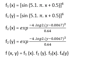
Maximizing f (x, y) is the same as minimizing - f (x, y)
- Now we are writing a code to find the Global maxima but before that, we are creating a separate function file which is labeled as a stalagmite, and then it is called by the main function where our program is executed and finds the global maxima of the given function.
function[f] = stalagmite(input_vector)

a = input_vector(1);
b = input_vector(2);
f1 = (sin((5.1*pi*a) +0.5))^6;
f2 = (sin((5.1*pi*b) +0.5))^6;
f3 = exp((-4*log(2)*((a-0.0667)^2))/(0.64));
f4 = exp((-4*log(2)*((b-0.0667)^2))/(0.64));
f = -[f1*f2*f3*f4];
end- The above program is saved as stalagmite in the database. To generate a stalagmite these are the above governing equations.
- The syntaxes for the 'ga ()’ command used in the above code.
- Now the first syntax is the basic genetic algorithm command where the ga () takes the inputs as a fitting equation that has to be evaluated and a number of variables present in the fitting function. So, each time this command is run it takes random values for the function variables initially and then uses those values for further calculations.
- The second syntax of ga () allows us to provide the bounds to the ga () command that will limit it, To choose the values within the specified values for the function variables. We can also give any linear inequalities and equalities as inputs and ga () will calculate according to these inequalities and equalities
- The third syntax of ga () gives the value of ‘x’ as well as the function’s minimum value. So, we can get a value of X where the function is minimum and that minimum value of the function is also calculated and given as output.
- Now the drawback of ga () command is it always calculates the value of x where the function is minimum, thus giving us the global minima. But we need to calculate global maxima in our code, so in order to achieve that we are minimizing the fitting function with a negative symbol because Maximizing f(x, y) is the same as minimizing -f(x, y). That is the reason we have put a negative symbol in the equation in the function code.
We are now writing the main program in MATLAB to optimize the stalagmite function and find the global maxima of the function:
%Program for genetic algorithm along with stalagmite function
clear all
close all
clc

%Defining search space
x = linspace(0,0.6,150); %Giving surface area of plot in x-direction
y = linspace(0,0.6,150); %Giving surface area of plot in x-direction
num_cases = 50; %number of times the GA runs

%Creating 2D array
[xx,yy] = meshgrid(x,y);

%Evaluating the stalagmite function generates the plot
for i = 1:length(xx);
    for j=1:length(yy);
     input_vector(1) = xx(i,j);
     input_vector(2) = yy(i,j);
     f(i,j) = stalagmite(input_vector);
    end
end

%CONVERTING FITTING FUNCTION TO CHANGE GRAPH UPWARDS
F = -f;


%plot 1
figure(1)
surf(xx,yy,F) %plot to visualise the function
shading interp
hold on


%PERFORMING GENETIC ALGORITHM
[output, fval] = ga(@stalagmite, 2,[],[],[],[],[0,0],[0.6,0.6])

%plotting global maxima
x_max = output(:,1);
y_max = output(:,2);
f_max = -fval;

plot3(x_max,y_max,f_max,'marker','o','MarkerSize',5,'MarkerFaceColor','r');
xlabel('X-VALUE')
ylabel('Y_VALUE')
title('STALAGMITE FUNCTION');
legend('stalagmite','globalmaxima')

%Study case:1 ie study of genetic algoritm unbounded

tic
for i = 1:num_cases
   [inputs,fopt(i)] = ga(@stalagmite,2);
   xopt(i) = inputs(1);
   yopt(i) = inputs(2);
end

Fopt = -fopt;

study1_time = toc;
figure(2)
subplot(2,1,1)
hold on
surf(xx,yy,F)
shading interp
plot3(xopt, yopt, Fopt,'Marker','o','MarkerSize',5,'MarkerFaceColor','r');
xlabel('X_values')
ylabel('Y_values')
title('UNBOUNDED INPUTS')
legend('stalagmite','globalmaxima')
subplot(2,1,2)
plot(Fopt)
title('Iterations in F')
xlabel('Iterations')
ylabel('Function Maximum')
legend('change in F values')

%Study case:2 ie study of genetic algoritm with upper and lower bounds

tic
for i = 1:num_cases
   [inputs,fopt(i)] = ga(@stalagmite,2,[],[],[],[],[0,0],[1,1]);
   xopt(i) = inputs(1);
   yopt(i) = inputs(2);
end

Fopt = -fopt;

study2_time = toc;
figure(3)
subplot(2,1,1)
hold on
surf(xx,yy,F)
shading interp
plot3(xopt, yopt, Fopt,'Marker','o','MarkerSize',5,'MarkerFaceColor','r');
xlabel('X_values')
ylabel('Y_values')
title('BOUNDED')
legend('stalagmite','globalmaxima')
subplot(2,1,2)
plot(Fopt)
title('variation in F')
xlabel('Iterations')
ylabel('Function Maximum')
legend('change in F values')

%Study case:3 ie Increasing GA population

options = optimoptions('ga');
options = optimoptions(options,'PopulationSize',200);

tic
for i = 1:num_cases
   [inputs,fopt(i)] = ga(@stalagmite,2,[],[],[],[],[0,0],[1,1],[],options);
   xopt(i) = inputs(1);
   yopt(i) = inputs(2);
end

Fopt = -fopt

study3_time = toc;
figure(4)
subplot(2,1,1)
hold on
surf(xx,yy,F)
shading interp
plot3(xopt, yopt, Fopt,'Marker','o','MarkerSize',5,'MarkerFaceColor','r');
xlabel('X_values')
ylabel('Y_values')
title('BOUNDED INPUTS AND INCREASING POPULATION')
legend('stalagmite','globalmaxima')
subplot(2,1,2)
plot(Fopt)
title('variation in F')
xlabel('Iterations')
ylabel('Function Maximum')
legend('change in F values')
CODE EXPLANATION:
- Here, first the commands close all, 'clear all 'clc, are used to close any previous plots and to clear the workspace and command window respectively
- Then the values of ‘x’ and ‘y’ are entered using the 'linspace()' command. This is our search space, which means for which value of x and y that are have defined in 'linspace() are we getting an optimized value for the stalagmite function.
- Using the 'mesh grid' command this 1-D array is converted into 2-D arrays. These 2-dimensional arrays are named xx and yy in the code.
- To calculate the stalagmite function we have used FOR LOOPS, and in these loops, we have defined 'i and j as each value of x and Y of the 2-dimensional array.
- Now for each value of 'X and y, we are creating an array named as 'input and thus this input will be a row vector i.e. two-column matrix.
- The first column of the input vector is defined as values of x matrix values and the second column of the input vector is defined as y matrix values.
- Using these values the stalagmite function is calculated. Function for the stalagmite is entered separately as a function code using the equations mentioned in above.
- The ga () function takes the 'input' values as the input for the function and returns the value of f. Now, the above function is called in the 'FOR LOOP for different values of X and y and different values of f are calculated.
These two 'FOR Loops’ generate the data for the plot that we need to generate a stalagmite graph.
Then ' the surface () command is used which creates a primitive, three-dimensional surface plot. If the command is entered as surface (X, Y, Z) then the function plots the values in matrix Z as heights above a grid in the the x-y plane defined by X and Y. The color of the surface varies according to the heights specified by Z. Here in this code (X.Y, Z) are (xx, yy, F) respectively
Then ‘shading interp' command is used to remove the grids that are formed on the plot, which will give us a smooth and better-looking plot.
Now to optimize the above function we used an inbuilt Matlab command called the 'ga(). This command performs the genetic algorithm on the function which we have defined and gives us output as optimized results. It will automatically perform the genetic algorithm calculations and give us the optimized solution for the fitting function as output.
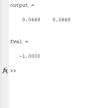
Now once we run the code, we will get a row vector for 'outputs' and the value of fval in the command window. The first value of the outputs vector is the value of X and the second value of the outputs vector is the value of y for which the value of the fitting function is minimum.
Now to plot the global maxima point in the graph we have defined value as x_max which is the first value of outputs vector and y value as y_max which is the second value of outputs vector.
As mentioned above, Maximizing flxy) is the same as minimizing-f(x, y), so since we have minimized the function-f. so the value of var' is the global maxima of the function. Since our graph is upward so the value of fval is multiplied by -symbol' and assigned to a variable f_max.
Then plot3() command is used as we need to plot point in a 3-d graph, global maxima is plotted using X_max. y_max and f_max.
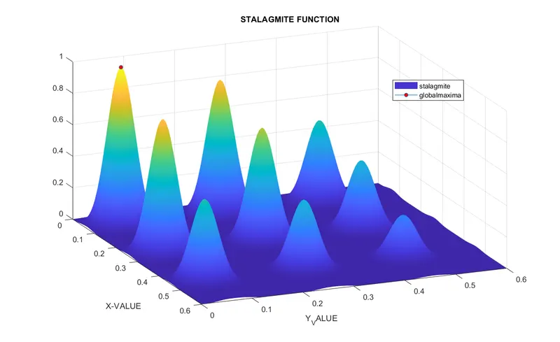
In the above Figure, we can observe that there are many local maxima in the plot, and the point gives us the global maxima of the function.
Output:
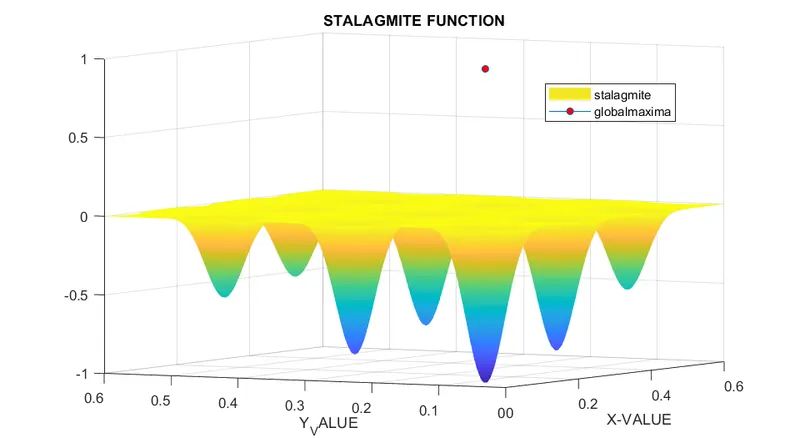
Error plot (a) without using -ve sign to the function
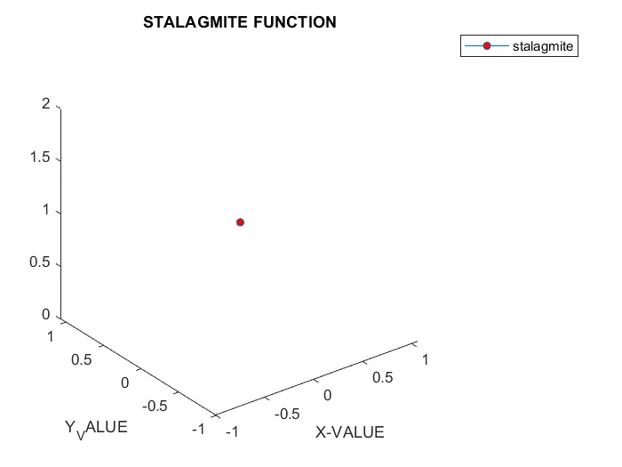
Error plot (b) without using hold command
Final plot showing the global maxima of the stalagmite:
To demonstrate how ga () works we have done 3 type of studies and coded it. The below programs and plots show us how to use genetic algorithm to obtain best results.
STUDY:1 STATISTICAL BEHAVIOUR
%Program for genetic algorithm along with stalagmite function
clear all
close all
clc

%Defining search space
x = linspace(0,0.6,150); %Giving surface area of plot in x-direction
y = linspace(0,0.6,150); %Giving surface area of plot in x-direction
num_cases = 50; %number of times the GA runs

%Creating 2D array
[xx,yy] = meshgrid(x,y);

%Evaluating the stalagmite function generates the plot
for i = 1:length(xx);
    for j=1:length(yy);
     input_vector(1) = xx(i,j);
     input_vector(2) = yy(i,j);
     f(i,j) = stalagmite(input_vector);
    end
end

%CONVERTING FITTING FUNCTION TO CHANGE GRAPH UPWARDS
F = -f;


%plot 1
figure(1)
surf(xx,yy,F) %plot to visualise the function
shading interp
hold on


%PERFORMING GENETIC ALGORITHM
[output, fval] = ga(@stalagmite, 2,[],[],[],[],[0,0],[0.6,0.6])

%plotting global maxima
x_max = output(:,1);
y_max = output(:,2);
f_max = -fval;

plot3(x_max,y_max,f_max,'marker','o','MarkerSize',5,'MarkerFaceColor','r');
xlabel('X-VALUE')
ylabel('Y_VALUE')
title('STALAGMITE FUNCTION');
legend('stalagmite','globalmaxima')

%Study case:1 ie study of genetic algoritm unbounded

tic
for i = 1:num_cases
   [inputs,fopt(i)] = ga(@stalagmite,2);
   xopt(i) = inputs(1);
   yopt(i) = inputs(2);
end

Fopt = -fopt;

study1_time = toc;
figure(2)
subplot(2,1,1)
hold on
surf(xx,yy,F)
shading interp
plot3(xopt, yopt, Fopt,'Marker','o','MarkerSize',5,'MarkerFaceColor','r');
xlabel('X_values')
ylabel('Y_values')
title('UNBOUNDED INPUTS')
legend('stalagmite','globalmaxima')
subplot(2,1,2)
plot(Fopt)
title('Iterations in F')
xlabel('Iterations')
ylabel('Function Maximum')
legend('change in F values')
CODE EXPLANATION:
This study shows us the statistical behavior of genetic algorithms in MATLAB.
- The code is similar to that of the above code, the only change here is that we are performing()' for some number of how iterations and see the values are changing for each iteration.
- In the above code, we have defined x and y values and then we have defined a number of times the ga ()' has to be variable num_cases and we have performed as a given it a value.
- Then using 'X and y we have created a 2-d array using the 'mesh grid()' command.
- Now above using code FOR used LOOP values of f are determined, it is same as the above code. Function code used here is also the same as the in this FOR LOOP.
- Now Since the values of f are negative and we will get a downward graph, in order to get an upward graph, we have multiplied f with the symbol and assigned it to a variable 'F
- Now another FOR LOOP is used to evaluate ga()' for 50 iterations. In this, FOR LOOP we have defined as the number of iterations and then we have entered the ga()' function with a normal syntax that we have mentioned in previous code. Only the fitting function and number of variables are entered as inputs for the ga(' functionThen the first value of inputs is assigned to a variable 'xopt and the second value of inputs is assigned to a variable 'yopt. Every time the FOR LOOP is executed it gives new values of fopt, xopt' and yopt.
- Then the 'fopt values are multiplied with '-symbol' and assigned to variable Fopt. This is done in order to point the global maxima since our graph will be upwards. This is only done for
- Now for this FOR LOOP plotting purpose. there is a command used 'tic and tok, this commands helps to know the time taken to calculate this FOR LOOP, tic is entered at the start for FOR LOOP and toc is entered after the ending of FOR LOOP and for 'toc a variable is assigned so the time is calculated under that variable.
- Then in 'figure()Y command is entered to open a figure window, then a 'subplot()' command is used to open the first graph in the figure window. Subplot(m,n.p) divides the current figure into an m -by- n grid and creates Accordingly the values are entered in the code axes in the position specified by p. for subplot()
- Then plotting is done using 'surface() command and then shading interp' is entered in the code to remove grids on the graph this first subplot. in the
- Then plot3() is used to generate a point in a 3-d graph, this command is used to plot the global maxima point. This helps us how we are getting the global maxima each and every time ga()' function is run.
- Then 'title()' command is used to give a title to the first plot, 'xlabel' and ylabel' commands are entered to name x-axis and y-axis respectively.
- Next, the second subplot command is entered to get the second graph between the optimized F values obtained from ga()" function and the number of iterations that 'ga()' is run.
- Then plot(" command is used to plot the graph between Fopt values and number of iterations.
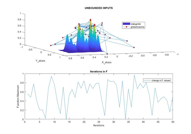
- Thus in the same figure window we will get two graphs using subplot( command).
- If we run the code, we will get above results, here we can observe that we have got different optimized values of function f each the ga() was run. We have got 50 different values of f when 50 times 'ga()' was run. So in this way, we can't use ga()' for our calculation in reality.
- We can observe the second graph in the figure that how values off are changing for each iteration.
- The genetic algorithm always takes random population samples and then performs the mutation and cross-over process to get a new generation. Due to these random inputs taken by the genetic algorithm, we get different values when we return gal() each time. Here genetic algorithm does not know what is our search space ie. limits of and y.
- To get better-optimized values of f' that are within the limits of x and y defined by us, we have used a modified ga()' syntax, which we will use in study 2
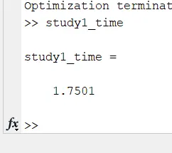
Now the 'tic and toc command entered in the code has calculated the time taken to finish whole FOR LOOP of the 'ga()' function and given us the time in the command window. It has taken nearly 2 seconds for ga() to generate the solution.
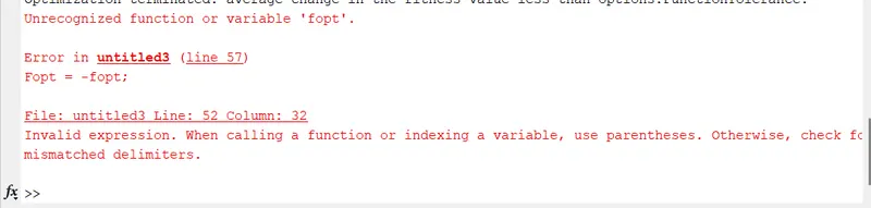
Error in commad window with out using the function input staligmite for study one
STUDY:2 STATISTICAL BEHAVIOUR WITH BOUNDED INPUTS
%Program for genetic algorithm along with stalagmite function
clear all
close all
clc

%Defining search space
x = linspace(0,0.6,150); %Giving surface area of plot in x-direction
y = linspace(0,0.6,150); %Giving surface area of plot in x-direction
num_cases = 50; %number of times the GA runs

%Creating 2D array
[xx,yy] = meshgrid(x,y);

%Evaluating the stalagmite function generates the plot
for i = 1:length(xx);
    for j=1:length(yy);
     input_vector(1) = xx(i,j);
     input_vector(2) = yy(i,j);
     f(i,j) = stalagmite(input_vector);
    end
end

%CONVERTING FITTING FUNCTION TO CHANGE GRAPH UPWARDS
F = -f;


%plot 1
figure(1)
surf(xx,yy,F) %plot to visualise the function
shading interp
hold on


%PERFORMING GENETIC ALGORITHM
[output, fval] = ga(@stalagmite, 2,[],[],[],[],[0,0],[0.6,0.6])

%plotting global maxima
x_max = output(:,1);
y_max = output(:,2);
f_max = -fval;

plot3(x_max,y_max,f_max,'marker','o','MarkerSize',5,'MarkerFaceColor','r');
xlabel('X-VALUE')
ylabel('Y_VALUE')
title('STALAGMITE FUNCTION');
legend('stalagmite','globalmaxima')

%Study case:2 ie study of genetic algoritm with upper and lower bounds

tic
for i = 1:num_cases
   [inputs,fopt(i)] = ga(@stalagmite,2,[],[],[],[],[0,0],[1,1]);
   xopt(i) = inputs(1);
   yopt(i) = inputs(2);
end

Fopt = -fopt;

study2_time = toc;
figure(3)
subplot(2,1,1)
hold on
surf(xx,yy,F)
shading interp
plot3(xopt, yopt, Fopt,'Marker','o','MarkerSize',5,'MarkerFaceColor','r');
xlabel('X_values')
ylabel('Y_values')
title('BOUNDED')
legend('stalagmite','globalmaxima')
subplot(2,1,2)
plot(Fopt)
title('variation in F')
xlabel('Iterations')
ylabel('Function Maximum')
legend('change in F values')
CODE EXPLANATION:
- The above code is the same as that of the previous code, only the change is in the syntax of the ga() command.
- Now in this code the syntax is used for ga() command is found in the range lb ≤ x ≤ ub.
Set A = [] and b = [] if no linear inequalities exist. Set Aeq=[] and beq=[] if no linear equalities exist.
- The above syntax helps us to enter upper and lower bound values as input to get a better solution than the previous code. This means that when ga() calculates the values of f, it will display on the values of F that lie between the bounded values of X and y
- Now it is not compulsory to take values of x and y values only as your bounded values, these values are taken according to the problem we are working on , sometimes for bounded values to be specified needs some practical experience for some situations. So bounded values are taken according to our problem.
- When we run the code we get the following figure,
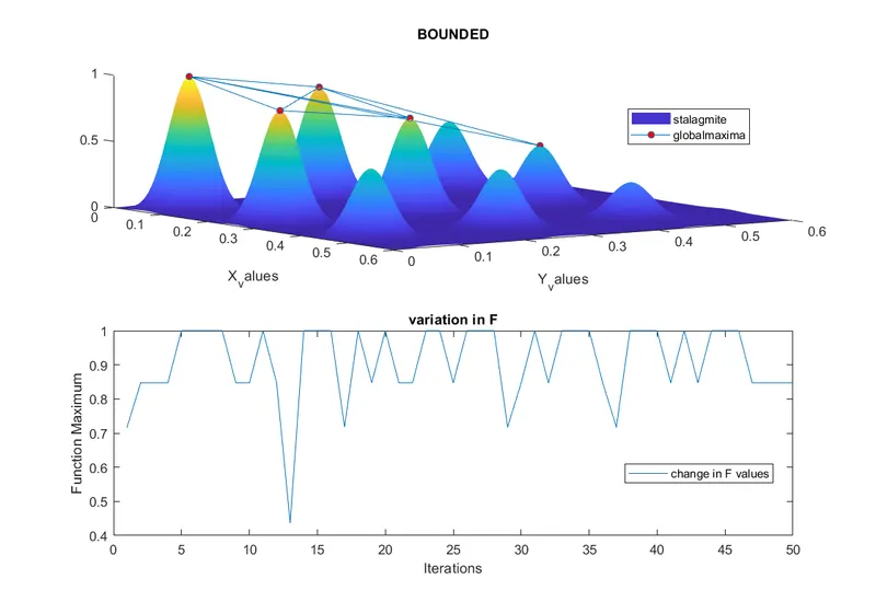
- In the above figure we can observe that now the graphs are much clear than the previous one and now, ga() predicts that the global maxima are somewhere between three points that are in the first plot.
- When you look at the second plot, we can also observe that our maximum value is between O.84 to 1
- But here still we didn’t get a single optimized value i.e. results are yet clear here. To overcome this problem, further, we are using the modified ga() command.
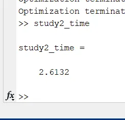
- In the above figure we can see that time taken by ga() to calculate is more compared to previous study. That means as we have entered more inputs ga() is taking more time to generate the solution.
Error in commad window with out using the function input staligmite for study two:

STUDY:3 STATISTICAL BEHAVIOUR WITH BOUNDED INPUTS AND INCREASED POPULATION:
clear all
close all
clc

%Defining search space
x = linspace(0,0.6,150); %Giving surface area of plot in x-direction
y = linspace(0,0.6,150); %Giving surface area of plot in x-direction
num_cases = 50; %number of times the GA runs

%Creating 2D array
[xx,yy] = meshgrid(x,y);

%Evaluating the stalagmite function generates the plot
for i = 1:length(xx);
    for j=1:length(yy);
     input_vector(1) = xx(i,j);
     input_vector(2) = yy(i,j);
     f(i,j) = stalagmite(input_vector);
    end
end

%CONVERTING FITTING FUNCTION TO CHANGE GRAPH UPWARDS
F = -f;


%plot 1
figure(1)
surf(xx,yy,F) %plot to visualise the function
shading interp
hold on


%PERFORMING GENETIC ALGORITHM
[output, fval] = ga(@stalagmite, 2,[],[],[],[],[0,0],[0.6,0.6])

%plotting global maxima
x_max = output(:,1);
y_max = output(:,2);
f_max = -fval;

plot3(x_max,y_max,f_max,'marker','o','MarkerSize',5,'MarkerFaceColor','r');
xlabel('X-VALUE')
ylabel('Y_VALUE')
title('STALAGMITE FUNCTION');
legend('stalagmite','globalmaxima')

%Study case:3 ie Increasing GA population

options = optimoptions('ga');
options = optimoptions(options,'PopulationSize',200);

tic
for i = 1:num_cases
   [inputs,fopt(i)] = ga(@stalagmite,2,[],[],[],[],[0,0],[1,1],[],options);
   xopt(i) = inputs(1);
   yopt(i) = inputs(2);
end

Fopt = -fopt

study3_time = toc;
figure(4)
subplot(2,1,1)
hold on
surf(xx,yy,F)
shading interp
plot3(xopt, yopt, Fopt,'Marker','o','MarkerSize',5,'MarkerFaceColor','r');
xlabel('X_values')
ylabel('Y_values')
title('BOUNDED INPUTS AND INCREASING POPULATION')
legend('stalagmite','globalmaxima')
subplot(2,1,2)
plot(Fopt)
title('variation in F')
xlabel('Iterations')
ylabel('Function Maximum')
legend('change in F values')
CODE EXPLANATION:
The code is the same as that of the previous two codes, the only change is in the ga() command, and one extra command is added to the code.
- In this code after the fitting function is calculated we have a command called 'optimoptions(). the syntax for this command is,
Options = optimoptions(SolverName) returns a set of default options for the SolverNamesolver. Options = optimoptions(SolverName,Name, Value) returns options with the named parameters altered with the specified values.
- This particular code helps us to rewrite the default values of any inbuilt MATLAB function. For the first syntax when we run it we will get all the default values of the solver function which is mentioned in the brackets. Here in our code, we have given ga in the brackets so this command will return default values of ga () function in MATLAB
- In the above figure we can see what the first syntax does. Here we can see that the default value for 'PopuationSize' is 50. That means when ga' takes random samples as inputs.it takes those values from a Population of 50, so the number of options to choose i for ga is less.
- If we increase this value of PopulationSize then ga will have more samples to choose and perform mutation and crossover then it can give us a more accurate optimized value.
- To change this value we used the second syntax of optimoptions() i.e. we have defined which solver the values have to change, then the parameter in that solver which has to be changed, and then by what value it has to be replaced.
- Thus by doing this we have changed the 'PopulationSize' to 200.
- Then, in the ga() function we have used the following syntax to give this change as one of the input,
x = ga(fun,nvars,A.b,Aeq.beq.lb.ub.nonlcon.options) minimizes with the default optimization parameters replaced by values in options. (Set nonlcon = [] if no nonlinear constraints exist.)
- Here in the above syntax we can enter all the inputs as that of previous code, additionally, we can also give nonlinear constraints and options' i.e. changes of defaults values as inputs in the ga() function.
- Since here we don't have any nonlinear constraints. We have entered in its place and we have entered the 'options' as input to tell the ga' that there is the change in the default values.
- Then the rest of the code is the same as the previous code and when we run this code we get the following results.
- From the above figure we can observe that by increasing the population size we have got a single optimized value in the first graph. If we increase the population size further, the value will be more accurate.
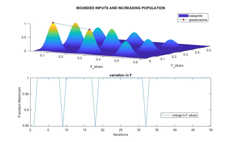
- In the second plot we can observe that the maximum value for many iterations is near 0.99999985 and only in three iterations ‘ga' predicts that values of f are less than of other iteration values. So the maximum value is somewhere near to this value. 14. This problem can be further rectified by increasing the population size and our graph will be much clearer.
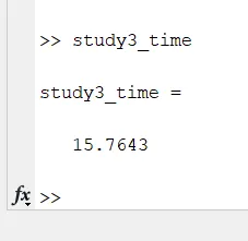
- Now we see in the command window that time taken by'ga’ function is more than that for previous codes. So as we increase the inputs'ga' takes more time to calculate. This is one of the drawback of 'gal()' command.
Error in commad window with out using the function input staligmite for study three:
CONCLUSION:
- The idea behind the above studies is to observe how the 'ga' command works with different inputs and how to obtain the same values for a function even if ga' is run several times.
- Thus global maxima is found for the stalagmite function.
- Genetic Algorithm process is one of the most used methods for obtaining optimized value.
- Genetic Algorithm is mostly used to find the minimum value of a function, for example, to find minimum drag force that will be created by the aerofoil
- Similar approach as above code can be used to find maximum values using ga command.