Challenge

Week 2- 2R Robotic Arm Challenge

SSarath Kumar M1 Feb 2022

Program to simulate the forward kinematics of 2R Robotic arm:

A 2R robotic arm contains two links and two rotational joints.

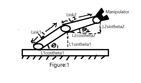
Considering a 2R robotic arm containing two Links which is attached to a manipulator.

Let the length of the Link1 be ‘L1’ and the length of the Link2 be 'L2'.

The initial point of link1 is attached to a base which makes an angle ‘θ1’ and the initial point of link2 is attached to final point of link1 which makes an angle ‘θ2’.

The end of Link2 is attached to a manipulator whose position has to be determined in the workspace. Hence;

By using Forward Kinematics;

To determine the final position of the manipulator in the workspace, when the angle ‘θ1’ and ‘θ2’ made by the links ‘L1’ and ‘L2’ are known; first we need to calculate the co-ordinates of the links L1 and L2 along x axis and y axis as follows;

Step:1

Calculating the position/co-ordinates of link1;

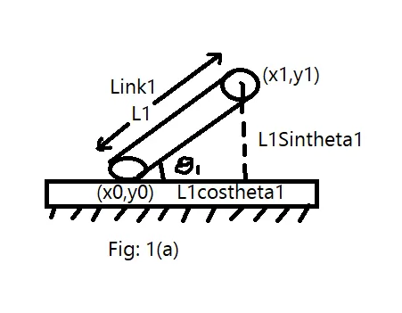
frm the fig 1(a);

Link L1 has two end points. i.e; initial point is connected to the base and the final/ending point of is connected to link 2. Hence the co-ordinate of the initial point is (0,0) and the co-ordinate of the final point of link l1 is (x1,y1)

Frm FHD of Link1;

x1 = L1cosθ1 and y1 = L1sinθ1

therefore; (x1,y1) = (L1cosθ1, L1sinθ1)

Step:2

Calculating the position/co-ordinate of link2;

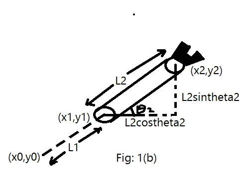
Link2 has two end points, where (x1,y1) is the initial point of link2 and (x2,y2) is the final position of link2.

From fig 1(b), Co-ordinates of link2 along x axis and y-axis are;

x2 = x1+L2cosθ2 and y2 = y1+L2sinθ2

Hence, the co-ordinates of the links L1 and L2 along x-axis and y-axis are;

[x0, y0] [x1,y1] [x2,y2]

With these co-ordinates we can plot the workspace of the manipulator using the below MatLab program by taking the inputs as follows;

Substituting the values of L1, L2 and θ1 and θ2, we get

clear all
close all
close all

%Inputs;
L1 = 1;
L2 = 0.5;

theta1 = 45;
theta2 = 30;

%co-ordinates
x0 = 0;
y0 = 0;

x1 = L1*cosd(theta1);
y1 = L1*sind(theta1);

x2 = x1 + L2*cosd(theta2);
y2 = y1 + L2*sind(theta2);

%plotting
line([x0 x1],[y0 y1],'linewidth',3,'color','b')
line([x1 x2],[y1 y2],'linewidth',3,'color','r')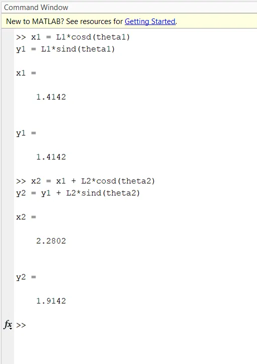

In the above prg, we have taken the inputs;

Length L1 = 1m; Length L2 = 0.5m

Angle made by Link1 wrt base θ1 = 45 Degree and Angle made by Link2 wrt Link1 θ2 = 30Degree

Using forward kinematics, Co-ordinates of L1 and L2:

[x0,y0] [x1,y1] [x2,y2]

Where; = x0 = 0 , y0 = 0;

x1 = L1*cosd(theta1) ; y1 = L1*sin(theta1)

x2 = x1 + L2*cos(theta2) ; y2 = y1 + L2*sin(theta2)

Here the program is executed only for a single time and determines the position of the manipulator at the required input angle in the workspace.

So we get;

x1 = (1)*cosd(45) = 1.4142

y1 = (1)*sind(45) = 1.4142

x2 = + 0.5*cosd(30) = 2.2802

y2 = + 0.5*sind(30) = 1.9142

So the co-ordinate/position of a 2R robotic arm with L1 = 1m and L2=0.5m at an angles 45 degree and 30 degree are

[0,0] [1.4142, 1.4142] [2.2802, 1.9142]

In the above program we can determine the position of the 2R robotic arm for a given particular value of θ. So, by using linspace command we can find the different position of the robotic arm in the workspace by providing the range of the angle of θ.

The program can be modified as follows;

Let us initialize the values of theta1 and theta2;

theta1 = linspace(0,90,10)

theta2 = linspace(0,90,10)

Here we are providing the range of the angle from 0 to 90 degrees with the length of 10. Which means that theta has 10 values within the range 0 to 90 degrees.

So, in order to to calculate the positions of the 2R robotic arm for multiple values of theta in a workspace, the program has to repeat, hence we are using for loop.

clear all
close all
close all

%Inputs;
L1 = 1;
L2 = 0.5;

theta1 = linspace(0,90,10);
theta2 = linspace(0,90,10);

for i = 1:length(theta1)
    THETA1 = theta1(i);
    for j = 1 : length(theta2)
        THETA2 = theta2(j);
x0 = 0;
y0 = 0;

x1 = L1*cosd(THETA1);
y1 = L1*sind(THETA1);

x2 = x1 + L2*cosd(THETA2);
y2 = y1 + L2*sind(THETA2);

%plotting
line([x0 x1],[y0 y1],'linewidth',3,'color','b')
line([x1 x2],[y1 y2],'linewidth',3,'color','r')

    end

end

for i = 1: length(theta1)

THETA1 = theta(i);

for j = 1: length(theta2)

THETA2 = theta(j);

end

For link1:

Number of values in theta1 is written as length(theta1)

Here we have considered the range of theta1 = linspace(0,90,10)

i.e; theta1 has a range from 0 to 90 degrees with 10 values.

So we are assigning the values to a variable ‘i’, to repeat the program as per the requirement.

for i = 1:10

we get;

i = 1 2 3 4 5 6 7 8 9 10

The logic here is we use the values of ‘i’ to take a particular value for theta1 then we assign each value of theta1 to a new variable THETA1.

Position of Link1 will be executed 10 times within the range 0 -90 degrees.

Also, for each value of THETA1 and each position of link1; link2 can take multiple position which depends on theta2. So we are using another ‘for loop’ for link2.

for j = 1:10

We get

j = 1 2 3 4 5 6 7 8 9 10

here, we use the values of ‘j’ to take a particular value for theta2. Again, each value of THETA1, will be looping to the values of theta2. then we assign each value of theta2 to a new variable THETA2.

Position of Link2 will be executed 10 times for each length of link1 within a range 0 -90 degrees. As shown in the below plot.

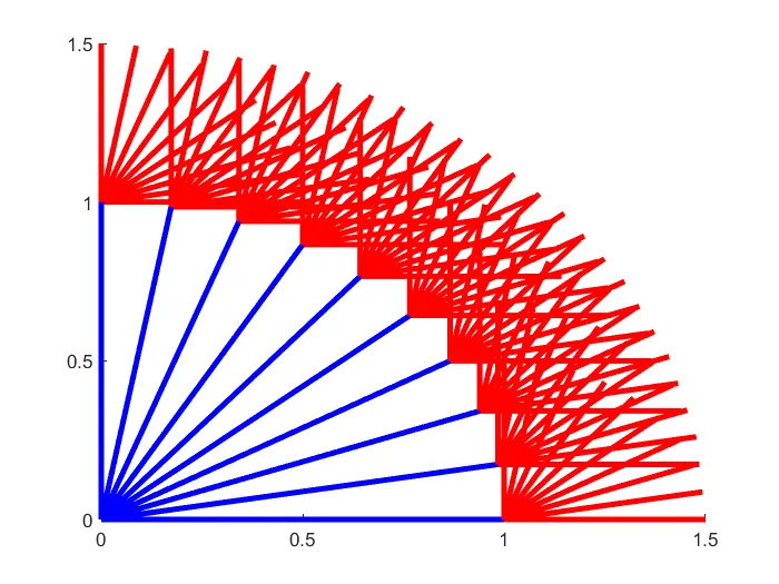
Here the position of 2R robotic arm is plotted at the same intervals for all angles of theta1 and theta2 in the workspace as shown in the above fig;

To plot the position of the 2R robotic arm for all the angles of theta1 and theta2 in different intervals can be obtained by using contour function.

Here, the contour functions usually execute the outputs for each angle of theta1 and theta2 which can be written by a below program.

clear all
close all
close all

%Inputs;
L1 = 1;
L2 = 0.5;

theta1 = linspace(0,90,4);
theta2 = linspace(0,90,4);

ct =1;
for i = 1:length(theta1)
    THETA1 = theta1(i);
    for j = 1 : length(theta2)
        THETA2 = theta2(j);
x0 = 0;
y0 = 0;

x1 = L1*cosd(THETA1);
y1 = L1*sind(THETA1);

x2 = x1 + L2*cosd(THETA2);
y2 = y1 + L2*sind(THETA2);

%plotting
figure(ct)
line([x0 x1],[y0 y1],'linewidth',3,'color','b')
line([x1 x2],[y1 y2],'linewidth',3,'color','r')
ct = ct+1;

    end

end

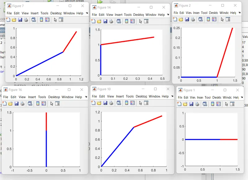
The program executes for each angle of theta1 and thetat2 plotting separately for given intervals as shown in the below fig, here the we obtain 16 plots representing the position of the manipulator for each angles of THETA1 and THETA2.

Further, by using hold on command also replacing co-ordinates of the line to plot command, we can plot each frame/output of the arm in the workspace into a video plot.

clear all
close all
close all

%Inputs;
L1 = 1;
L2 = 0.5;

theta1 = linspace(0,90,4);
theta2 = linspace(0,90,4);

ct =1;
for i = 1:length(theta1)
    THETA1 = theta1(i);
    for j = 1 : length(theta2)
        THETA2 = theta2(j);
x0 = 0;
y0 = 0;

x1 = L1*cosd(THETA1);
y1 = L1*sind(THETA1);

x2 = x1 + L2*cosd(THETA2);
y2 = y1 + L2*sind(THETA2);

%plotting
hold on
plot([x0 x1],[y0 y1],'linewidth',3,'color','b')
plot([x1 x2],[y1 y2],'linewidth',3,'color','r')
pause(0.3)
ct = ct+1;

    end

end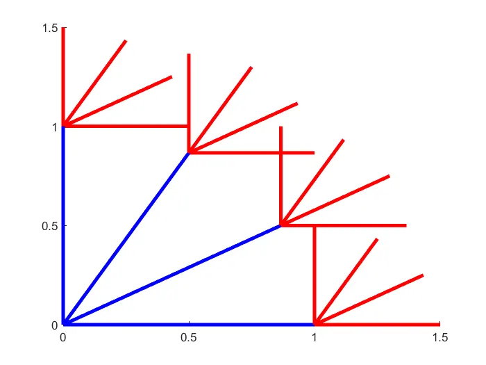

We are now combining all the co-ordinates into a single plot command so that we get a plot into a video file/ animation consisting of each frame of the 2R robotic along the workspace.

clear all
close all
close all

%Inputs;
L1 = 1;
L2 = 0.5;

theta1 = linspace(0,90,40);
theta2 = linspace(0,90,40);

ct =1;
for i = 1:length(theta1)
    THETA1 = theta1(i);
    for j = 1 : length(theta2)
        THETA2 = theta2(j);
x0 = 0;
y0 = 0;

x1 = L1*cosd(THETA1);
y1 = L1*sind(THETA1);

x2 = x1 + L2*cosd(THETA2);
y2 = y1 + L2*sind(THETA2);

%plotting
plot([x0 x1],[y0 y1],[x1 x2],[y1 y2],'linewidth',3)
axis([-0.1 1.5 0 1.5])
pause(0.03)
ct = ct+1;

    end

end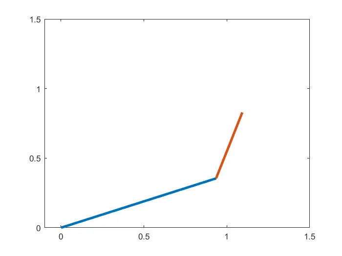

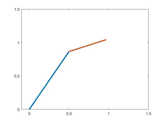
To execute the program which can plot the position of the manipulator in the form a video, we use the below profram and the logic is explained as follows;

% Forward kinematics of 2D Robotic arm manipulator:

clear all
close all
clc

% inputs
l1 = 1;
l2 = 0.5;

theta1 = linspace(0,90,10);
theta2 = linspace(0,90,10);

ct = 1;
for i = 1:length(theta1)
    THETA1 = theta1(i);

    for j =1:length(theta2)
        THETA2 = theta2(j);

        x0 = 0;
        y0 = 0;

        x1 = l1*cosd(THETA1);
        y1 = l1*sind(THETA1);

        x2 = x1 + l2*cosd(THETA2);
        y2 = y1 + l2*sind(THETA2);

%plotting
plot([x0 x1],[y0 y1],[x1 x2], [y1 y2],'linewidth',3)
axis([-0.1 1.5 0 1.5])
pause(0.03)
M(ct) = getframe(gcf);
ct=ct+1;

    end

end

movie(M)
videofile = VideoWriter('Forward_kinematics.avi','Uncompressed AVI');
open(videofile)
writeVideo(videofile,M)
close(videofile)

Here we get an animation of the 2R arm in the screen. In order to save the file and visualize all the frame like a movie we use an array ‘M’ where each frame ‘ct’ is stored then we transfer the frame data to a function getframe where the frames are saved as gcf.

Now we write a logic to get an animation of the frames which is stored in ‘M’.

Now, we are creating a videofile wherein the data/file is saved as Forward_kinematics in the form of avi.

Which can be written as ;

videofile = VideoWriter('Forward_kinematics.avi','Uncompressed AVI');

Now, we are using a function called writevideo which is used to combine the array data [‘M’] and the saved videofile. After executing the program we get a video file with a animation representing the position of the 2R robotic arm in the workspace.

Plot: Refer below You tube link to find the plot of the program.

https://youtu.be/ya90QjUTKYc

Week 2- 2R Robotic Arm Challenge

Ship work like this
in your own course.

Talk to a career counsellor

Ship work like thisin your own course.

Talk to a career counsellor

Ship work like this
in your own course.