Exhaust Port Challenge

Aim: To Simulate the Conjugate heat transfer analysis using exhaust port model also calculate the wall and surface heat transfer coefficient values of the model

Theory:

Conjugate heat transfer: The Conjugate Heat Transfer (CHT) analysis type allows for the simulation of heat transfer between solid and fluid domains by exchanging thermal energy at the interfaces between them. Typical applications of this analysis type exist as, but are not limited to, the simulation of heat exchangers, cooling of electronic equipment, and general-purpose cooling and heating systems.

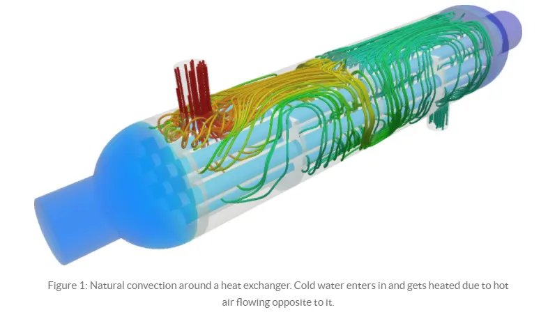
Conjugate heat transfer corresponds with the combination of heat transfer in solids and heat transfer in fluids. In solids, conduction often dominates whereas in fluids, convection usually dominates. Conjugate heat transfer is observed in many situations. For example, heat sinks are optimized to combine heat transfer by conduction in the heat sink with the convection in the surrounding fluid.

Heat Transfer by Solids and Fluids

Heat Transfer in a Solid

In most cases, heat transfer in solids, if only due to conduction, is described by Fourier’s law defining the conductive heat flux, q, proportional to the temperature gradient: .

For a time-dependent problem, the temperature field in an immobile solid verifies the following form of the heat equation:

Heat Transfer in a Fluid

Due to the fluid motion, three contributions to the heat equation are included:

1. The transport of fluid implies energy transport too, which appears in the heat equation as the convective contribution. Depending on the thermal properties on the fluid and on the flow regime, either the convective or the conductive heat transfer can dominate.
2. The viscous effects of the fluid flow produce fluid heating. This term is often neglected, nevertheless, its contribution is noticeable for fast flow in viscous fluids.
3. As soon as a fluid density is temperature-dependent, a pressure work term contributes to the heat equation. This accounts for the well-known effect that, for example, compressing air produces heat.

Accounting for these contributions, in addition to conduction, results in the following transient heat equation for the temperature field in a fluid:

Conjugate Heat Transfer Applications

Effective Heat Transfer

Efficiently combining heat transfer in fluids and solids is the key to designing effective coolers, heaters, or heat exchangers.

The fluid usually plays the role of energy carrier on large distances. Forced convection is the most common way to achieve high heat transfer rate. In some applications, the performances are further improved by combining convection with phase change (for example liquid water to vapour phase change).

Even so, solids are also needed, in particular to separate fluids in a heat exchanger so that fluids exchange energy without being mixed.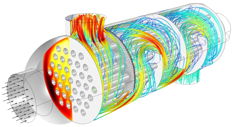

Flow and temperature field in a shell-and-tube heat exchanger illustrating heat transfer between two fluids separated by the thin metallic wall.

Heat sinks are usually made of metal with high thermal conductivity (e.g. copper or aluminum). They dissipate heat by increasing the exchange area between the solid part and the surrounding fluid.

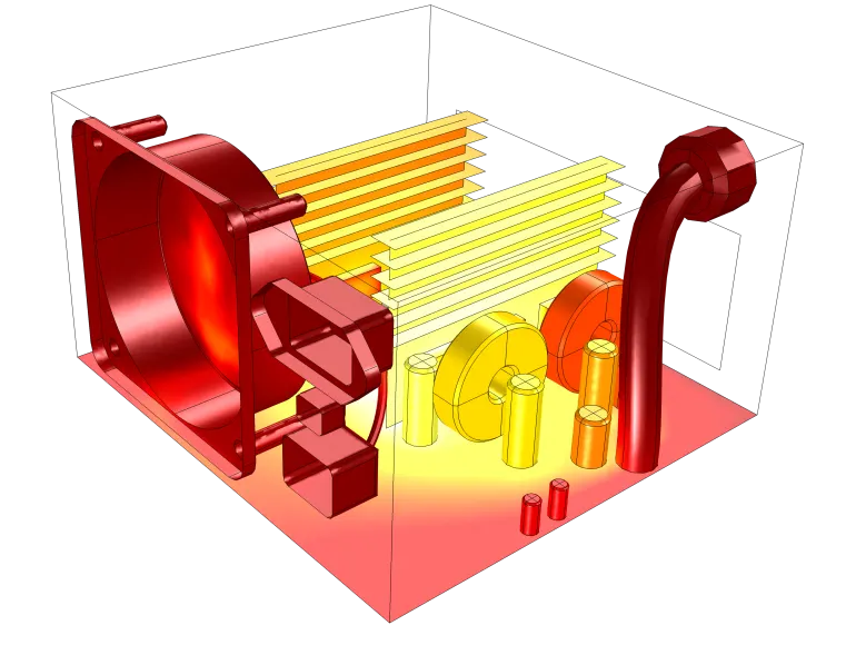
Temperature field in a power supply unit cooling due to an air flow generated by an extracting fan and a perforated grille. Two aluminum fins are used to increase the exchange area between the flow and the electronic components.

Energy Savings

Heat transfer in fluids and solids can also be combined to minimize heat losses in various devices. Because most gases (especially at low pressure) have small thermal conductivities, they can be used as thermal insulators… provided they are not in motion. In many situations, gas is preferred to other material due to its low weight. In any case, it is important to limit the heat transfer by convection, in particular by reducing the natural convection effects. Judicious positioning of walls and use of small cavities helps to control the natural convection. Applied at the micro scale, the principle leads to the insulation foam concept where tiny cavities of air (bubbles) are trapped in the foam material (e.g. polyurethane), which combines high insulation performances with light weight.

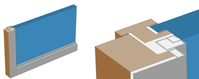
Window cross section (left) and zoom-in on the window frame (right).

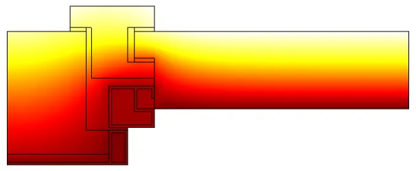
Temperature profile in a window frame and glazing cross section from ISO 10077-2:2012 (thermal performance of windows).

Fluid and Solid Interactions

Fluid/Solid Interface

The temperature field and the heat flux are continuous at the fluid/solid interface. However, the temperature field can rapidly vary in a fluid in motion: close to the solid, the fluid temperature is close to the solid temperature, and far from the interface, the fluid temperature is close to the inlet or ambient fluid temperature. The distance where the fluid temperature varies from the solid temperature to the fluid bulk temperature is called the thermal boundary layer. The thermal boundary layer size and the momentum boundary layer relative size is reflected by the Prandtl number : for the Prandtl number to equal 1, thermal and momentum boundary layer thicknesses need to be the same. A thicker momentum layer would result in a Prandtl number larger than 1. Conversely, a Prandtl number smaller than 1 would indicate that the momentum boundary layer is thinner than the thermal boundary layer. The Prandtl number for air at atmospheric pressure and at 20°C is 0.7. That is because for air, the momentum and thermal boundary layer have similar size, while the momentum boundary layer is slightly thinner than the thermal boundary layer. For water at 20°C, the Prandtl number is about 7. So, in water, the temperature changes close to a wall are sharper than the velocity change.

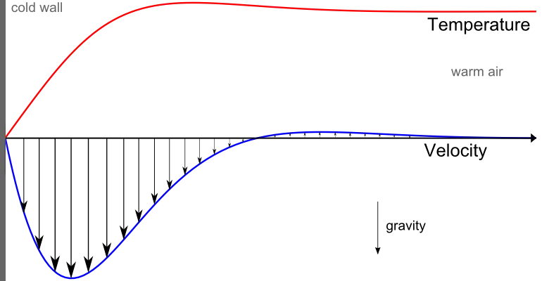
Normalized temperature (red) and velocity (blue) profile for natural convection of air close to a cold solid wall.

Natural Convection

The natural convection regime corresponds to configurations where the flow is driven by buoyancy effects. Depending on the expected thermal performance, the natural convection can be beneficial (e.g. cooling application) or negative (e.g. natural convection in insulation layer).

The Rayleigh number, noted as , is used to characterized the flow regime induced by the natural convection and the resulting heat transfer. The Rayleigh number is defined from fluid material properties, a typical cavity size, , and the temperature difference,, usually set by the solids surrounding the fluid:

The Grashof number is another flow regime indicator giving the ratio of buoyant to viscous forces:

The Rayleigh number can be expressed in terms of the Prandtl and the Grashof numbers through the relation .

When the Rayleigh number is small (typically <10³), the convection is negligible and most of the heat transfer occurs by conduction in the fluid.

For a larger Rayleigh number, heat transfer by convection has to be considered. When buoyancy forces are large compared to viscous forces, the regime is turbulent, otherwise it is laminar. The transition between these two regimes is indicated by the critical order of the Grashof number, which is 10⁹. The thermal boundary layer, giving the typical distance for temperature transition between the solid wall and the fluid bulk, can be approximated by  when  is of order 1 or greater.

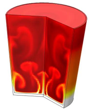
Temperature profile induced by natural convection in a glass of cold water in contact with a hot surface .

Forced Convection

The forced convection regime corresponds to configurations where the flow is driven by external phenomena (e.g. wind) or devices (e.g. fans, pumps) that dominate buoyancy effects.

In this case the flow regime can be characterized, similarly to isothermal flow, using the Reynolds number as an indicator,. The Reynolds number represents the ratio of inertial to viscous forces. At low Reynolds numbers, viscous forces dominate and laminar flow is observed. At high Reynolds numbers, the damping in the system is very low, giving small disturbances. If the Reynolds number is high enough, the flow field eventually ends up in turbulent regime.

The momentum boundary layer thickness can be evaluated, using the Reynolds number, by .

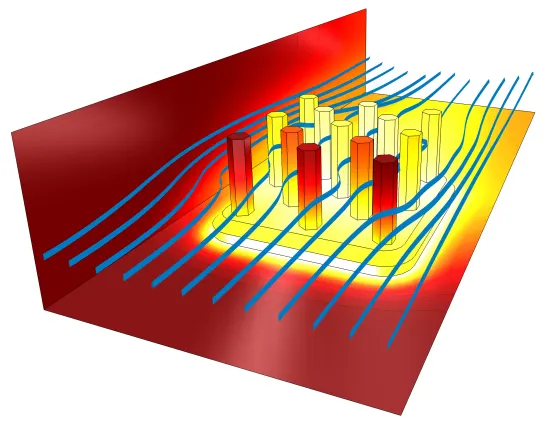
Streamlines and temperature profile around a heat sink cooling by forced convection.

Radiative Heat Transfer

Radiative heat transfer can be combined with conductive and convective heat transfer described above.

In a majority of applications, the fluid is transparent to heat radiation and the solid is opaque. As a consequence, the heat transfer by radiation can be represented as surface-to-surface radiation transferring energy between the solid wall through transparent cavities. The radiative heat flux emitted by a diffuse gray surface is equal to . When a surface is surrounded by bodies at a homogeneous , the net radiative flux is . When surrounding surfaces of different temperatures, each surface-to-surface exchange is determined by the surface’s view factors.

Nevertheless, both fluids and solids may be transparent or semitransparent. So radiation can occur in fluid and solids. In participating (or semitransparent) media, the radiation rays interact with the medium (solid or fluid) then absorb, emit, and scatter radiation.

Whereas radiative heat transfer can be neglected in applications with small temperature differences and lower emissivity, it plays a major role in applications with large temperature differences and large emissivities.

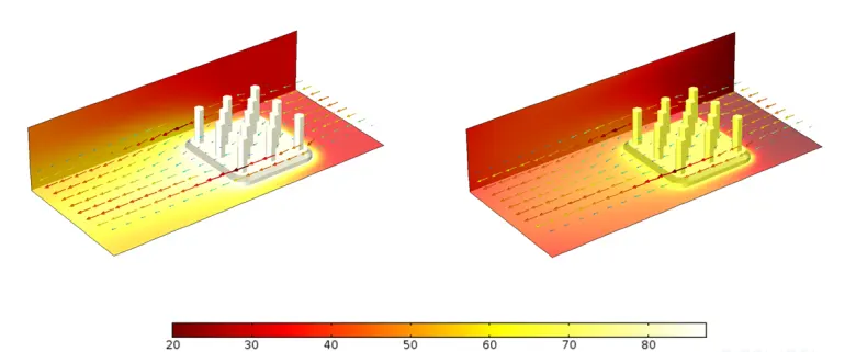
Comparison of temperature profiles for a heat sink with a surface emissivity  (left) and  (right).

Conclusion

Heat transfer in solids and heat transfer in fluids are combined in the majority of applications. This is because fluids flow around solids or between solid walls, and because solids are usually immersed in a fluid. An accurate description of heat transfer modes, material properties, flow regimes, and geometrical configurations enables the analysis of temperature fields and heat transfer. Such a description is also the starting point for a numerical simulation that can be used to predict conjugate heat transfer effects or to test different configurations in order, for example, to improve thermal performances of a given application.

Notations

: heat capacity at constant pressure (SI unit: J/kg/K)

: gravity acceleration (SI unit: m/s²)

: Grashof number (dimensionless number)

: thermal conductivity (SI unit: W/m/K)

: characteristic dimension (SI unit: m)

: refractive index (dimensionless number)

: absolute pressure (SI unit: Pa)

: Prandtl number (dimensionless number)

: heat flux (SI unit: W/m²)

: heat source (SI unit: W/m³)

: Rayleigh number (dimensionless number)

: strain rate tensor (SI unit: 1/s)

: temperature field (SI unit:K)

: ambient temperature (SI unit: K)

: velocity field (SI unit: m/s)

: typical velocity magnitude (SI unit: m/s)

: thermal expansion coefficient (SI unit: 1/K)

: momentum boundary layer thickness (SI unit: m)

: thermal layer thickness (SI unit: m)

: characteristic temperature difference (SI unit: K)

: surface emissivity (dimensionless number)

: density (SI unit: kg/m³)

: Stefan-Boltzmann constant (SI unit: W/m²T⁴)

: viscous stress tensor (SI unit: N/m²)

 Geometry:

First open the geometry file in Space Claim, after check the any extra edges are their or not?, if their use the repair options or remove the extra edges.

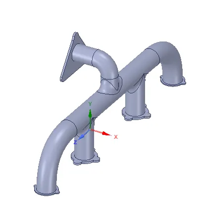
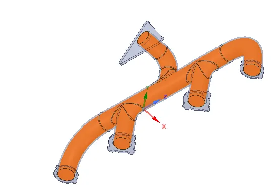
Next create the volume region in the geometry, after share the topology of the geometry for creating a conformal mesh which will give the accurate results of the solution.

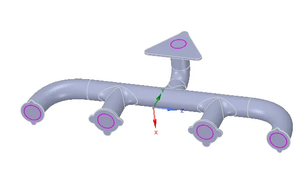
                                   Final Geometry

 Base line Simulation:

Mesh:

  

    

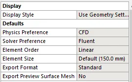
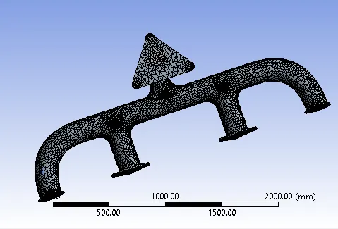
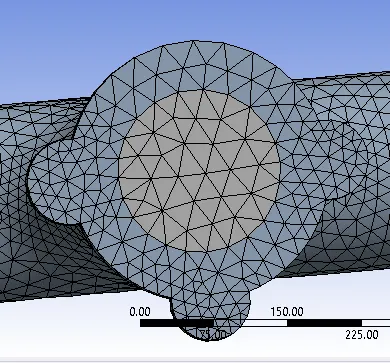
Setup:

Solver:

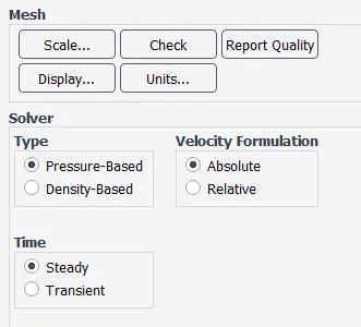
Model:

Energy equation is on

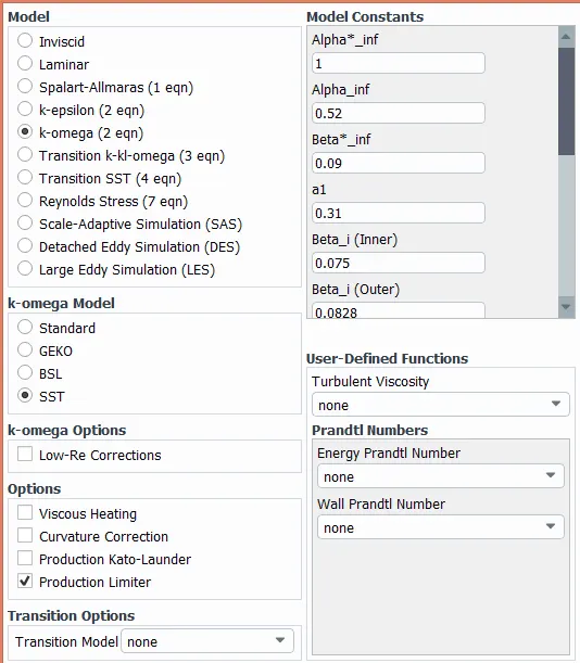
K-omega SST model

Materials:

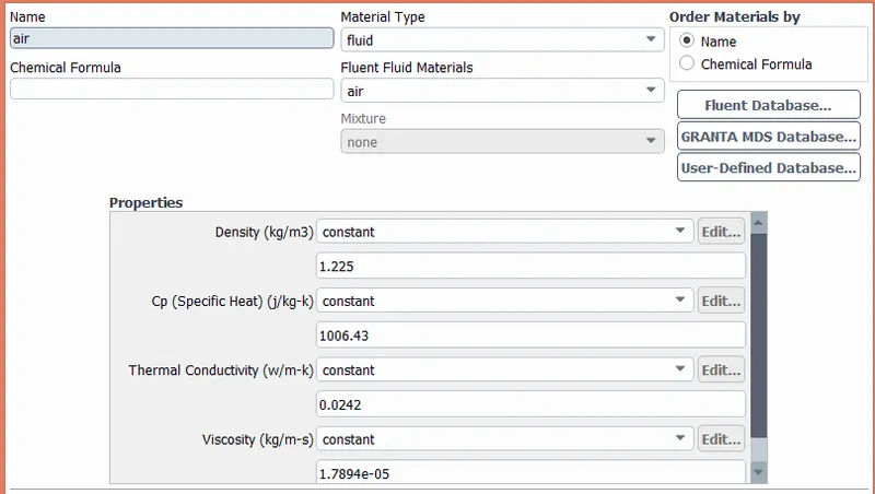
Fluid: air

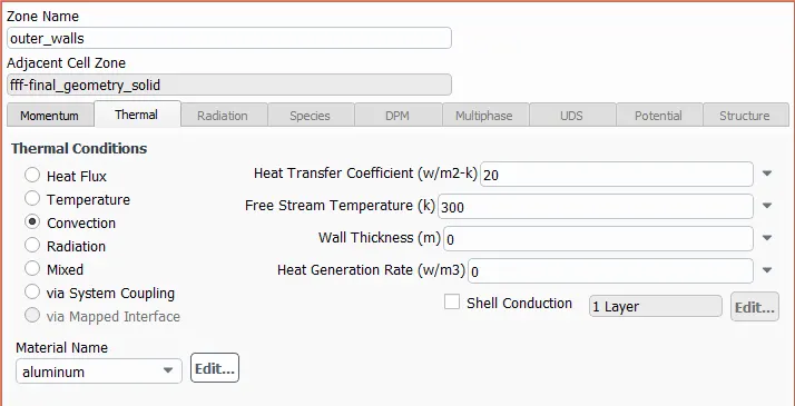
Solid : Aluminium

Boundary Conditions:

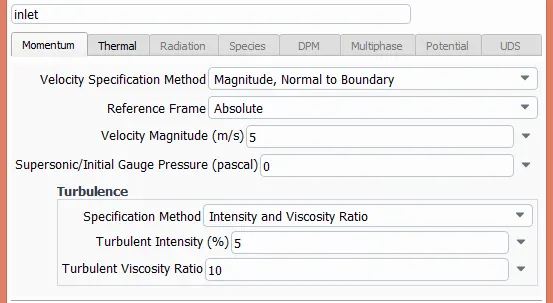
Inlet:

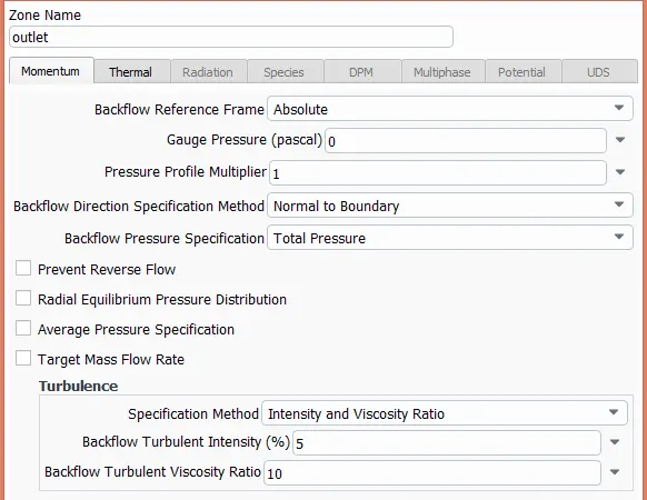
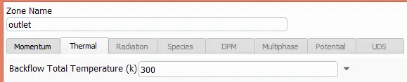
Outlet:

Wall Function:

Initialization:

Plots:

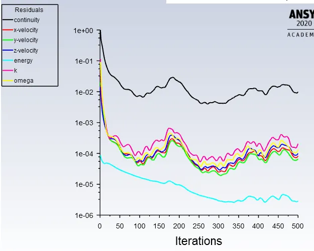
Residual plot:

Post Processing:

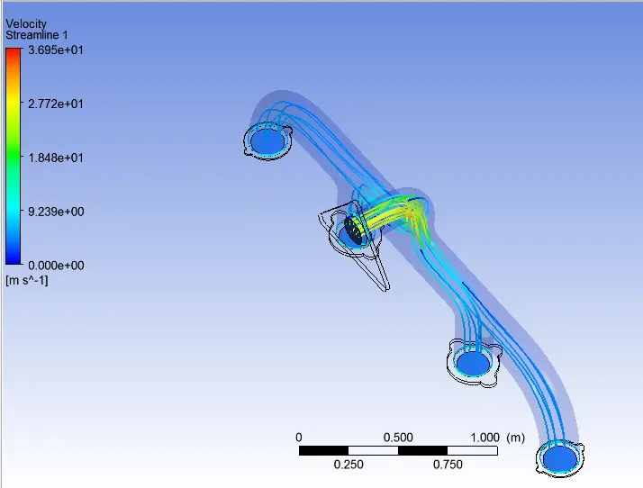
Velocity Steamline:

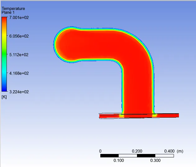
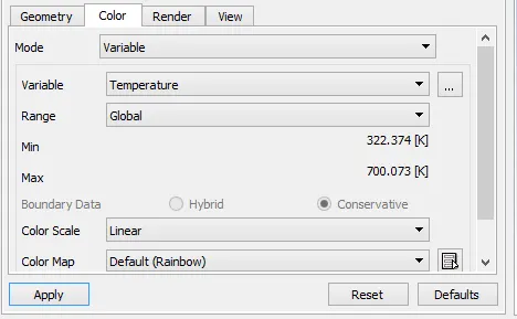
Temperature Contour:

Velocity Contour:

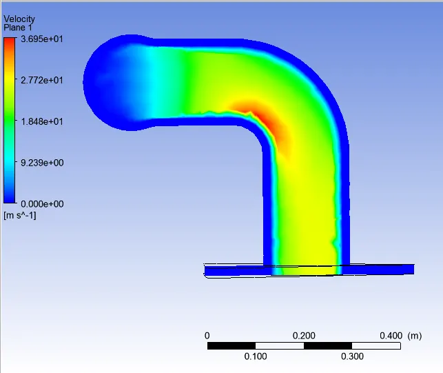
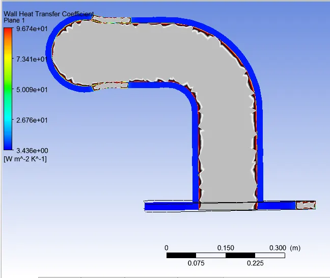
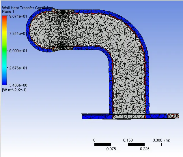
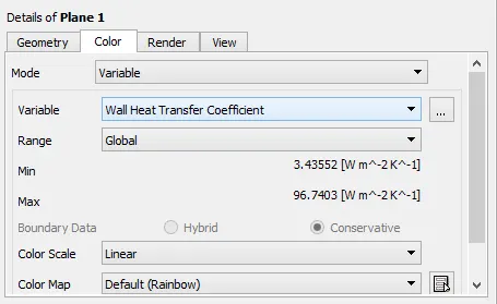
Wall Heat transer coefficent:

Pressure contour:

Conclusions:

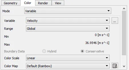
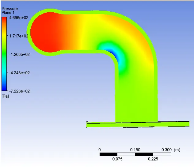
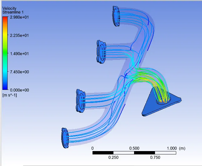
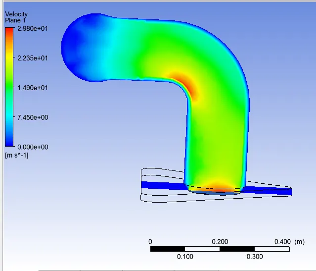
the above graph velocity is maximum at the bend (36.9546m/s). because near the turning the pressure decreases and the velocity increases as the fluid moves towards the outlet. Also minimum pressure can be seen at bend of the contour.

In an exhaust port analysis the hot air enters into the inlet and then it transfers heat from the convection to the exhaust port body and then it transfer heat through the condction all along the body of the part.

Here the base line mesh, the temperature of exhaust port should rise when all the inlets combine with each other near the outlet bend pipe.

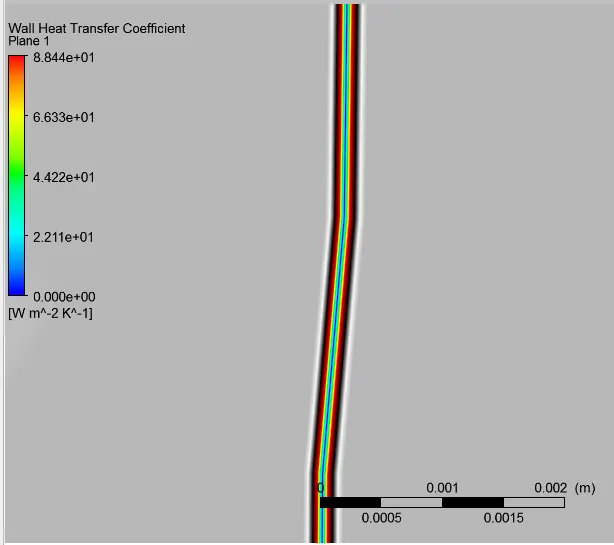
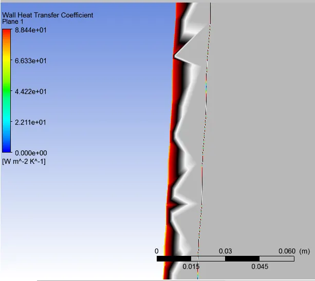
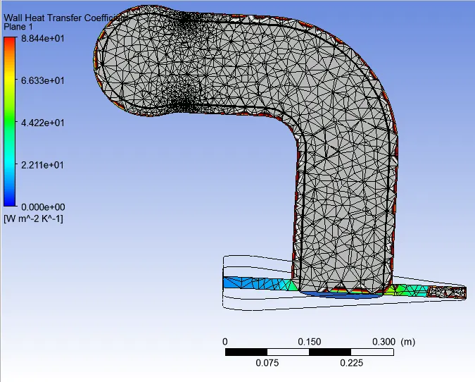
The plot of wall heat transfer coefficent is not smoother because of coaser mesh near the wall. for getting the smoother curve inflation layers are used.

In inflation layers first calculate the first layer thickness values with the help of Y+ values.

Due to low renolds number the Y+ value is in between 0 to 5, so K- omega SST is best suitable model for this simulation.

The maximum Temperature can be seen the entire outlet bend pipe 

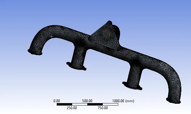
Reinement mesh:

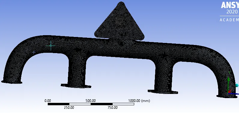
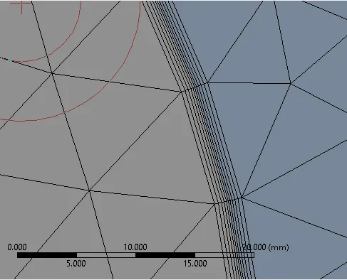
In refined mesh the whole geometry and setup will be same.Here we will change the mesh and we will redefine the mesh by giving the proper boundary layer mesh sizes by providing the inflation layer size according to the turbulence model.

If you want to capture the flow near the walls where the flow has reynolds number we will be using K-Omega boundary condition with y+ value between 1-5.

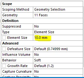
For the refinement we will provide the inflation layer by giving the first layer thickness of the lnflation layer. Apart from that we will setup body sizing or the extracted fluid volume with the size of 10mm. 

Inflation Layers:

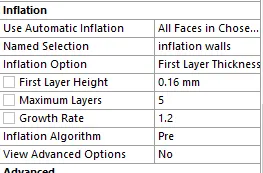
In the inflation layer the first layer thickness of 0.16mm and with the number of layers 5 growth rate be 1.2. 

or getting the total thickness of the inflation layers we are taking Y+ = 5(for k-Omega SST model Y+ in between 0 to 5)

Calculating total thickness value

 

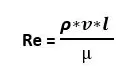
     Re = 1.225*5*1.044/1.89e-05

           = 680555.55

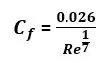
         = 0.026/(680555.555)^1/7

         = 0.003817

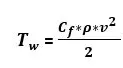
          = 0.003817*1.225*(5)^2/2

          = 0.05845

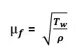
         = 0.24174

      = 100*1.89e-05/00.24174*1.225

      = 0.16mm

Plots:

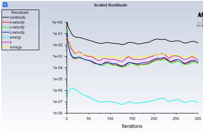
Residual Plot:

Contours:

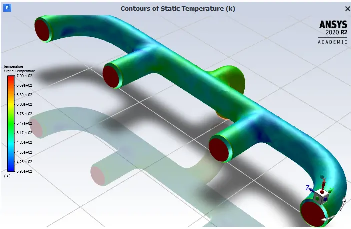
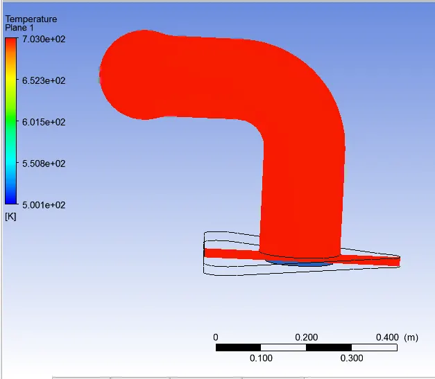
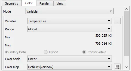
Temperature contour

 Velocity Steam line :

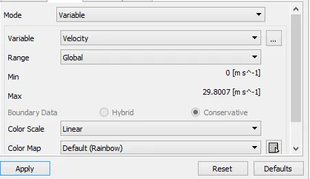
Velocity Profile:

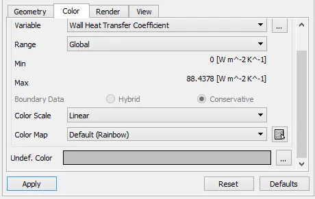
Heat transfer coefficent:

Pressure Contour:

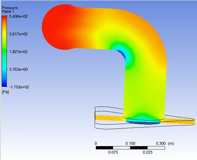
Here we performed the simulation for both the cases and we thus get the velocity, temperature and pressure contours.

Both the cases there  are no change in temperature difference .

Inflation layers have been added along the boundary of the fluid and solid volume thus capturing the accurate boundary layers according to the K-omega SST model.

Heat transfer is higher between fluid and solid at outlet because the velocity of the fluid is higher.

How would you verify if the HTC predictions from the simulations are right? On what factors does the accuracy of the prediction depend on

The results for the simulation can be validated either by some experimental results and then manually calculation out the data for result validation.

Mesh: The proper gird size is required for capturing the boundary layer.

Proper inflation layer and edge sizing is highly required for solving the problem.

Turbulence model: Proper turbulence model should be chosen wisely for the problem to capture the different required phenomenon, according to Y+ value setup.

for capturing phenomenon near the wall (low Reynolds number) K-Omega method is suitable.(Y+ = 1-5)

for capturing phenomenon flow away from the wall(high Reynolds number) K-epsilon method is suitable.(Y+ = 30-300)

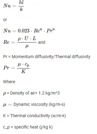
By theoretical calculation of Nusselt number to find the heat transfffer coefficient.

Nusselt Number: it is the ratio of heat transferred through convection to the heat transfer through conduction.

this will tell about how much the heat transfer is enhanced due to fluid motion.

Factors does the accuracy depends on

Mesh Refinement

No of Inflation layers

Choose the right turbulence model(Y+ value)