Curve fitting using Matlab

Aim: Writing a code for fit a linear and cubic polynomial for the cp data.

Theory:

Curve fitting is a process of constructing a curve, or mathematical functions, which possess the closest proximity to the real series o data. By curve fitting, we can mathematically construct the functional relationship between the observed dataset and parameter values, etc.

The accuracy of the curve fit can be improved by increasing the degree of the polynomial.

so, Best fit can obtained by increasing the degree of the polynomial.

Perfect fit:

The perfect fit is achieved when the geometric distances from the given points to the fitting curve is zero. This means that the curve fits perfectly on the points.

To get a perfect fit we can increase to a order of the polynomials.

Best fit:

The perfect fit is achieved when the geometric distances from the given points to the fitting curve is minimized. in the least suares sense.Finding the best fit reduces to the minimization of the objective function where denotes the fitting curve.

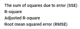
Parameters used to measure the curve fitting charactersitics:

Software Used: MATLAB PROGRAMMING

Program: Linear curve fit

clear all
close all
clc

% Data Preparation

cp_data = load('data'); % data file having values of temperatura and specific heats values
temperature = cp_data(:,1);
cp = cp_data(:,2);

% curve fit
% cp = a*T^2 + b*T +c

co_effs = polyfit(temperature,cp,1)
predicted_cp = polyval(co_effs,temperature);

% ploting the graphs

plot(temperature,cp,'linewidth',3)
hold on
plot (temperature,predicted_cp,'linewidth',3 ,'color','r')
xlabel('Temperature [K]')
ylabel('Specific Heat [KJ/Kmole-K]')
legend('original data','curve fit')

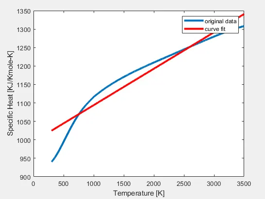
Output Graph:

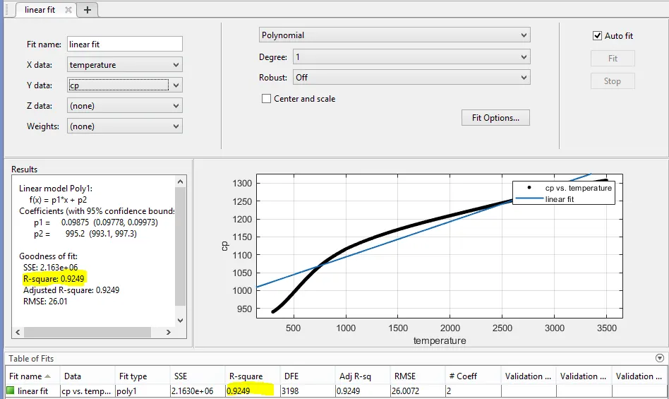
Curve Fitting tool for linear fit:

Conclusions:

R-square is lies in 0.9249 not in between (0.95 to 1), so it is not a best possible curve fit.

Program:Cubic curve fit

clear all
close all
clc

% Data Preparation

cp_data = load('data'); % data file having values of temperatura and specific heats values
temperature = cp_data(:,1);
cp = cp_data(:,2);

% curve fit
% cp = a*T^2 + b*T +c

co_effs = polyfit(temperature,cp,3)
predicted_cp = polyval(co_effs,temperature);

% ploting the graphs

plot(temperature,cp,'linewidth',3)
hold on
plot (temperature,predicted_cp,'linewidth',3 ,'color','r')
xlabel('Temperature [K]')
ylabel('Specific Heat [KJ/Kmole-K]')
legend('original data','curve fit')

Output Plot

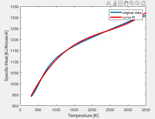
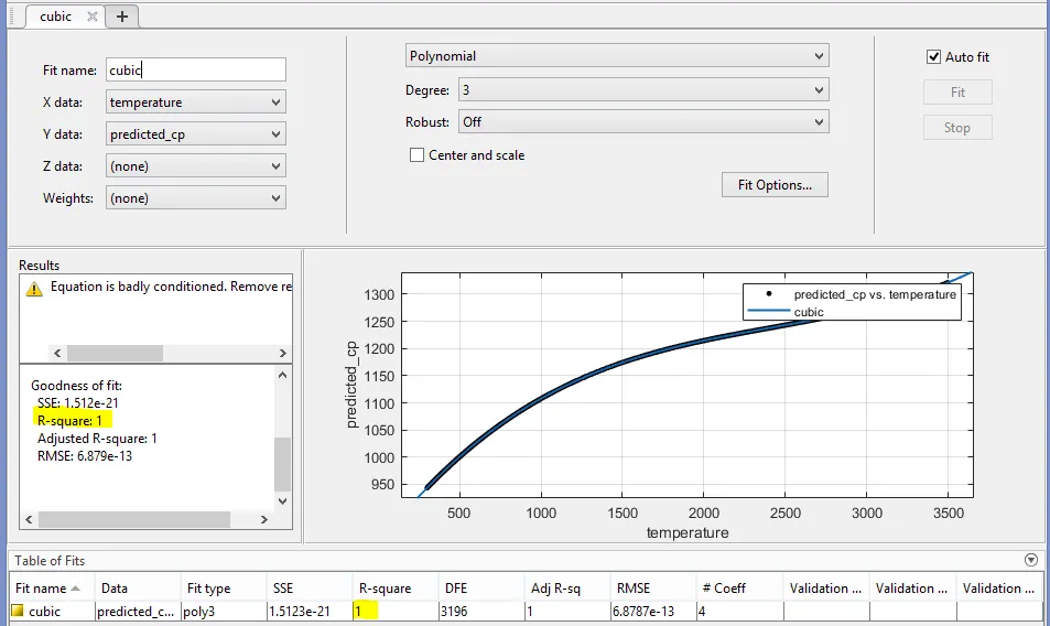
Curve Fiting for cubic fit:

Conculsion:

R-square is lies in 1 so it a best possible curve fit.

Program:Split-wise fit

% Split wise curve fit

clear all
close all
clc

% Data Preparation

cp_data = load('data'); % data file having values of temperatura and specific heats values
temperature = cp_data(:,1);
cp = cp_data(:,2);

% curve fit

co_eff1 = polyfit(temperature(1:1600),cp(1:1600),3);
co_eff2 = polyfit(temperature(1600:3000),cp(1600:3000),3);

predicted_cp1 = polyval(co_eff1,temperature(1:1600));
predicted_cp2 = polyval(co_eff2,temperature(1600:3000));

% ploting the graphs

plot(temperature,cp,'linewidth',3)
hold on
plot (temperature(1:1600),predicted_cp1,'linewidth',3 ,'color','r')
plot (temperature(1600:3000),predicted_cp2,'linewidth',3 ,'color','g')

xlabel('Temperature [K]')
ylabel('Specific Heat [KJ/Kmole-K]')
legend('original data','curve fit','split-wise fit')
title('split-wise curve fit')

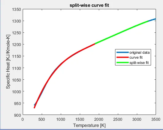
Output graph:

Conclusion:

The accuracy of the curve fit will can be provided by increase the degree of the polynomial.

1.How to make a curve fit perfectly:

In Perfect fit, without showing the centering error and scaling error, the curve fit should fit the original curve in that particular order of the polynomial.

2.How to get the best fit:

for getting a best fit , we can check the parameters of the characteristic curve fitting. we can increase the order of polynomial to get the best fit.

we can use the split-wise method to get best fit.

3.What could be done to imrove the cubic fit:

By using the Split-wise method, we can improve a curve fit for that particular order of polynomial.

we must split the original data set into some small ranges, such that we should different co-efficent for the curve fit functions for the small ranges.

after combining the values, we can plot the entire data.

Note:

Therory reference taken by the skill-lync videos portal