Week 8: Literature review - RANS derivation and analysis

Aim: The objective of the project is apply Reynolds decomposition to the Navier-Strokes equation and determine the expression of Reynolds stress.

Theory:

The Reynolds-averaged Navier–Stokes equations (or RANS equations) are time-averaged[a] equations of motion for fluid flow. The idea behind the equations is Reynolds decomposition, whereby an instantaneous quantity is decomposed into its time-averaged and fluctuating quantities, an idea first proposed by Osborne Reynolds.[1] The RANS equations are primarily used to describe turbulent flows. These equations can be used with approximations based on knowledge of the properties of flow turbulence to give approximate time-averaged solutions to the Navier–Stokes equations. For a stationary flow of an incompressible Newtonian fluid, these equations can be written in Einstein notation in Cartesian coordinates as:

The left hand side of this equation represents the change in mean momentum of a fluid element owing to the unsteadiness in the mean flow and the convection by the mean flow. This change is balanced by the mean body force, the isotropic stress owing to the mean pressure field, the viscous stresses, and apparent stress owing to the fluctuating velocity field, generally referred to as the Reynolds stress. This nonlinear Reynolds stress term requires additional modeling to close the RANS equation for solving, and has led to the creation of many different turbulence models.

Reynolds Decomposition:

REYNOLDS AVERAGED NAVIER-STOKES EQUATIONS

By hand of a time-averaging of the NS equations and the continuity equation for incompressible fluids, the basic equations for the averaged turbulent flow will be derived in the following. The flow field can then be described only with help of the mean values.
In order to be able to take a time-average, the momentary value is decomposed into the parts mean value and fluctuating value. This is shown graphically in Figure 1

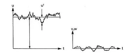
Figure 1

The momentary velocity components is u , the time-averaged value is named and the fluctuating velocity has the letter u′ . With help of this definition the decomposition can mathematically be written as:

Eq-1

Analogously for the density and the temperature:

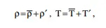Eq-2

which will however be considered constant in the following.

The chosen averaging method takes the mean values at a fix place in space and averaged over a time span that is large enough for the mean values to be independent of it.

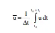Eq-3

The time-averaged values of the fluctuating values are defined to be zero:

Eq-4

Firstly the continuity equation is averaged. If we substitute the expressions for the velocities from Eq-1 into the continuity equation we get:

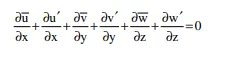Eq-5

The time-average of the last equation is written as:

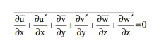Eq-6

Before we look at the transformation and reduction of Eq-6, a summary of rules for time averaging shall be given:

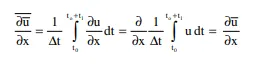Eq-7

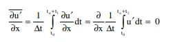
Eq-8

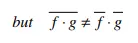
The averaged derivatives of the fluctuations are also zero according to these rules, so that the time averaged continuity equation is:

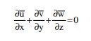Eq-9

Now the NS equations will be time-averaged. The averaging will be exemplified for the x-component. Beforehand a small transformation of the advection term.

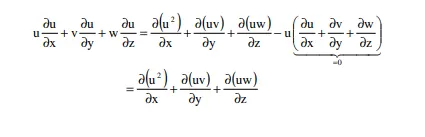Eq-10

The expressions for the decomposition of the velocities from Eq-1 are now substituted into the transformed Navier-Stokes equation and a time-average is done:

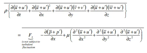Eq-11

Application of the rules from Eq-7 and Eq-8 shows that among others the terms

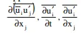
from the equation above can be reduced and the equation can be transformed to:

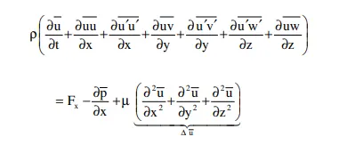Eq-12

Further small transformations, for example a repeated application of the product rule and the continuity equation to the advection term, lead to a form of the time-averaged NS equations for all three directions as:

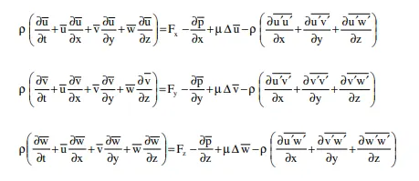Eq-13

Or in tensor form:

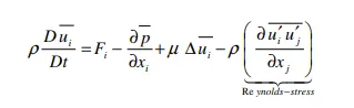Eq-14

From now on the time-averaged fields will not be over lined anymore. So for example u stands for the time-averaged velocity component in direction of the x-axis.
We pay attention to the last two terms of the right side of Eq-14:

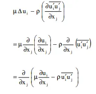Eq-15

The expression in the brackets above corresponds to the total shear stress:

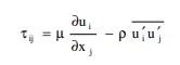Eq-16

If we compare to the Navier-Stokes equations, it is conspicuous that besides the viscous part an additional term has been added to the total shear stress. This term results from the time-average and is generally the dominant part of the total shear stress. Since the term only appears due to the Reynolds average, it is called Reynolds stress or apparent turbulent shear stress.

As stated in the introduction to the RANS approach, to lead to the closure of the equation system, an approximation for the Reynolds stresses has to be done, which sets in relation the apparent shear stresses with the velocity field of the average flow.

Reynolds Stress:

In fluid dynamics, the Reynolds stress is the component of the total stress tensor in a fluid obtained from the averaging operation over the Navier–Stokes equations to account for turbulent fluctuations in fluid momentum.

Turbulent viscosity:

The turbulent transfer of momentum by eddies creates internal fluid friction. It is the fundamental idea of how we define viscosity in turbulent flow, i.e. internal fluid resistance. Eddy viscosity explains what causes the internal friction.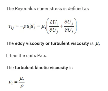

Molecular viscosity:

Molecular viscosity is the same as viscosity. The Coefficient of Molecular Viscosity is the same value as dynamic viscosity. Molecular viscosity is the transport of mass motion momentum solely by the random motions of individual molecules not moving together in coherent groups. Molecular viscosity is analogous in laminar flow to eddy viscosity in turbulent flow.

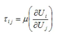
It is the resistance to the movement of one layer of fluid over an adjacent layer of fluid.

It is linear and easy to measure.

It is a Fluid property.

The flow is laminar and smooth. It is dominant in laminar flow regimes, where the Reynolds number is low.

The velocity of flow is generally low and he molecular viscosity depends on the thickness of the fluid.

Turbulent Viscosity:

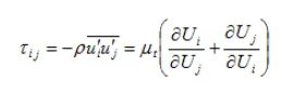
It is a function of fluctuations in velocity in velocity term and is influenced by disorderliness inflow.

It is a non-linear and difficult to estimate.

It is dependent on flow domains such as velocity, Reynolds number.

It is not a fluid property.

The flow of turbulence is not smooth due to eddies and swirl.

It is dominant in turbulent flow regimes, where the Reynolds number is high.

The velocity of flow is high and the turbulent viscosity depends on the velocity and flow conditions of the fluid.