Week 6: Conjugate Heat Transfer Simulation
Aim: Simulate the Conjugate heat transfer analysis for flow through a pipe with diffrent mesh sizes.
Study the Effect of super cycle stages intervals.
Software Used: Converge CFD
Theory:
Conjugate heat transfer: The Conjugate Heat Transfer (CHT) analysis type allows for the simulation of heat transfer between solid and fluid domains by exchanging thermal energy at the interfaces between them. Typical applications of this analysis type exist as, but are not limited to, the simulation of heat exchangers, cooling of electronic equipment, and general-purpose cooling and heating systems.
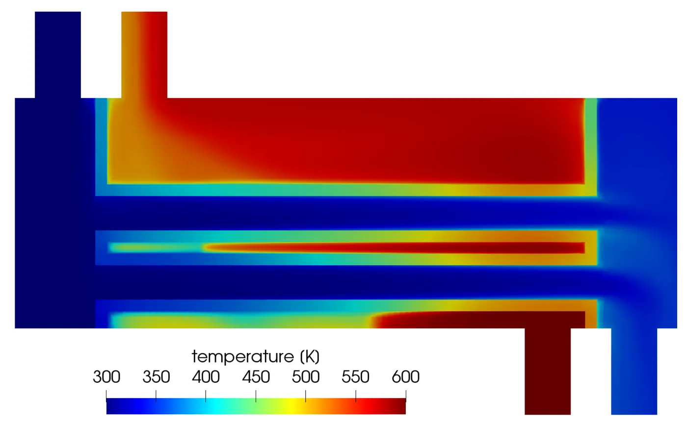
Conjugate heat transfer corresponds with the combination of heat transfer in solids and heat transfer in fluids. In solids, conduction often dominates whereas in fluids, convection usually dominates. Conjugate heat transfer is observed in many situations. For example, heat sinks are optimized to combine heat transfer by conduction in the heat sink with the convection in the surrounding fluid.
Heat Transfer by Solids and Fluids
Heat Transfer in a Solid
In most cases, heat transfer in solids, if only due to conduction, is described by Fourier’s law defining the conductive heat flux, q, proportional to the temperature gradient:  .
.
For a time-dependent problem, the temperature field in an immobile solid verifies the following form of the heat equation:

Heat Transfer in a Fluid
Due to the fluid motion, three contributions to the heat equation are included:
- The transport of fluid implies energy transport too, which appears in the heat equation as the convective contribution. Depending on the thermal properties on the fluid and on the flow regime, either the convective or the conductive heat transfer can dominate.
- The viscous effects of the fluid flow produce fluid heating. This term is often neglected, nevertheless, its contribution is noticeable for fast flow in viscous fluids.
- As soon as a fluid density is temperature-dependent, a pressure work term contributes to the heat equation. This accounts for the well-known effect that, for example, compressing air produces heat.
Accounting for these contributions, in addition to conduction, results in the following transient heat equation for the temperature field in a fluid:

Super Cycling:
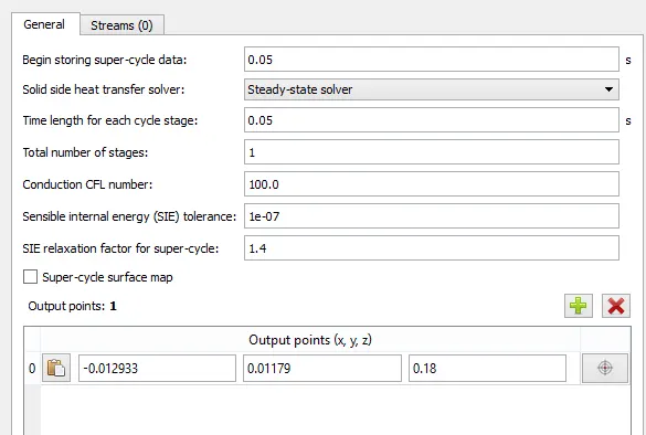
Super-cycling is a method used by CONVERGE Studio in the case of conjugate heat transfer problems with a solid and liquid regions.
The integral problem here is that both solvers cannot run at the same speed since solving in the fluid domain is much faster owing to the time scale difference for heat transfer in liquids as compared to solids. This causes problems during the solution given that the solid side solver would not have reached a steady state/convergence in the time the liquid solver does. This is where the concept of super-cycling can be used.
The basic idea of super-cycling is that the solver for the fluid domain is paused until the solver for the solid domain converges. This pausing is done in intervals that can be set by the user and will be explained below.
Geometry Creation:
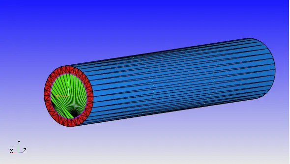
Calculation of velocity using Reynolds number:

Given Re = 7000
Properties of Air:
Density = 1.225 kg/m3
Dynamic viscosity = 1.89*10e-5 kg/m-s
D = 0.04 m
Therefore V = 2.7m/s
Case Setup:
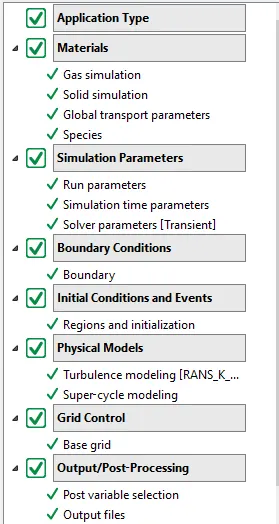
Application type:

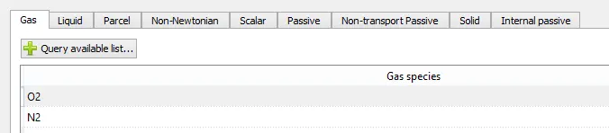
Materials: Air
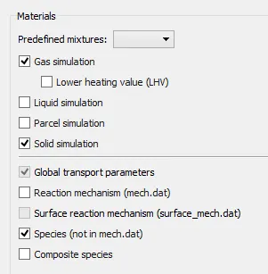
Solid Simulation: Aluminium as solid Material
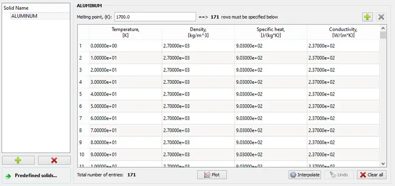
Species:
Solid:

Gas:
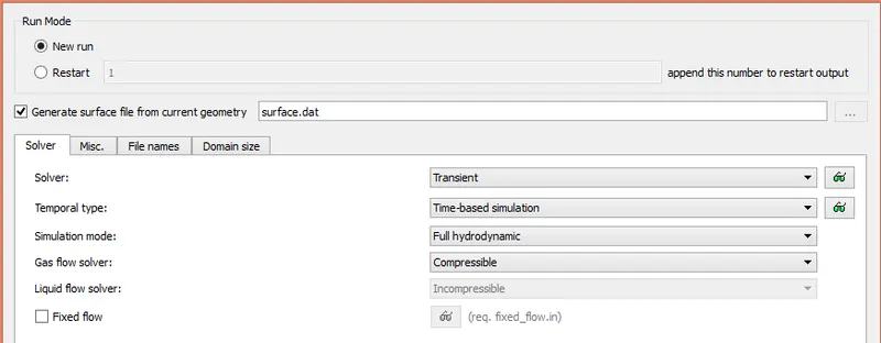
Run Parameters:
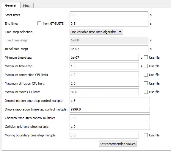
Simulation time Parameters:
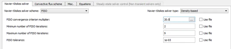
Solver Parameters:
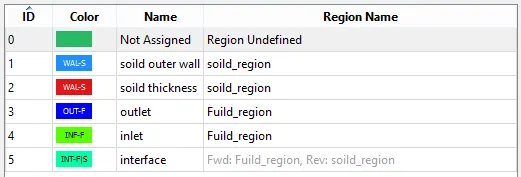
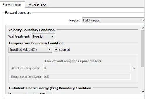
Boundary Conditions:
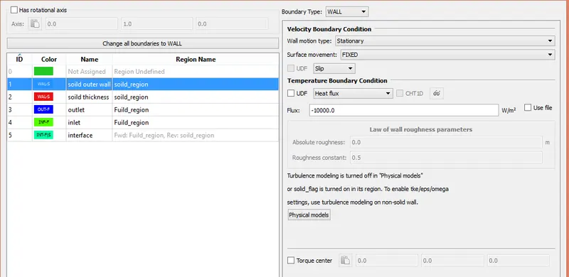
Solid outer walls:
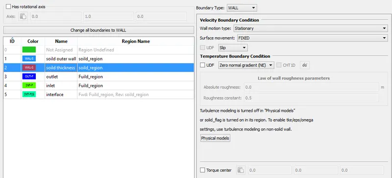
Solid Thickness walls:
Inlet:
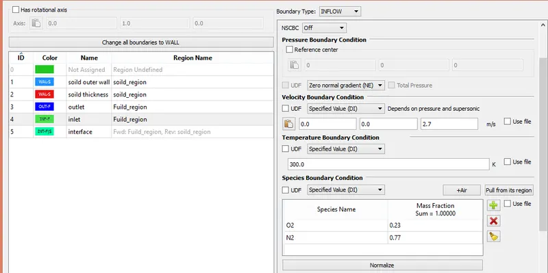
Outlet:
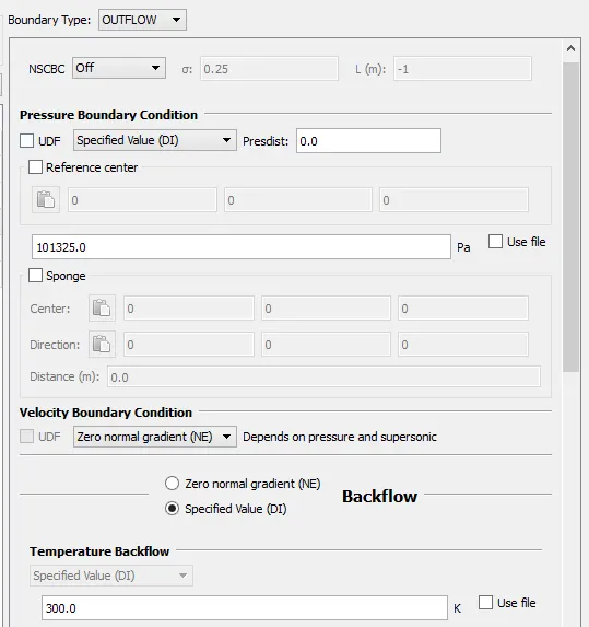
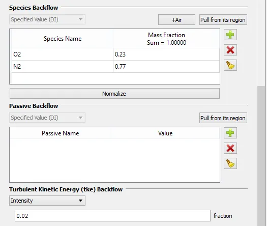
Interface:
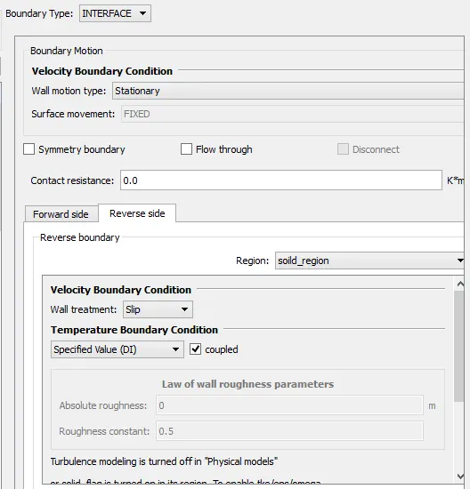
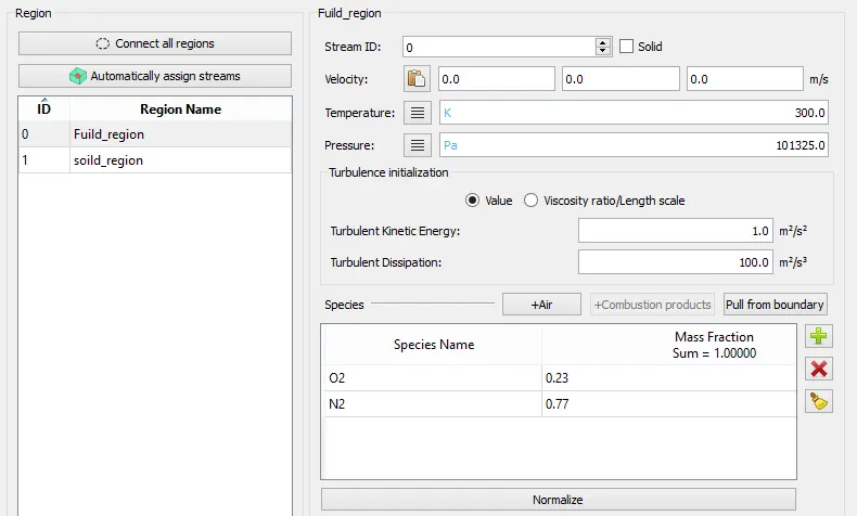
Initial Conditions:
Fluid Region:
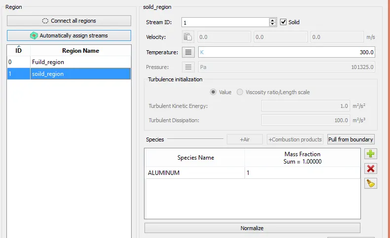
Solid Region:
Physical Models:
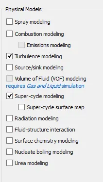
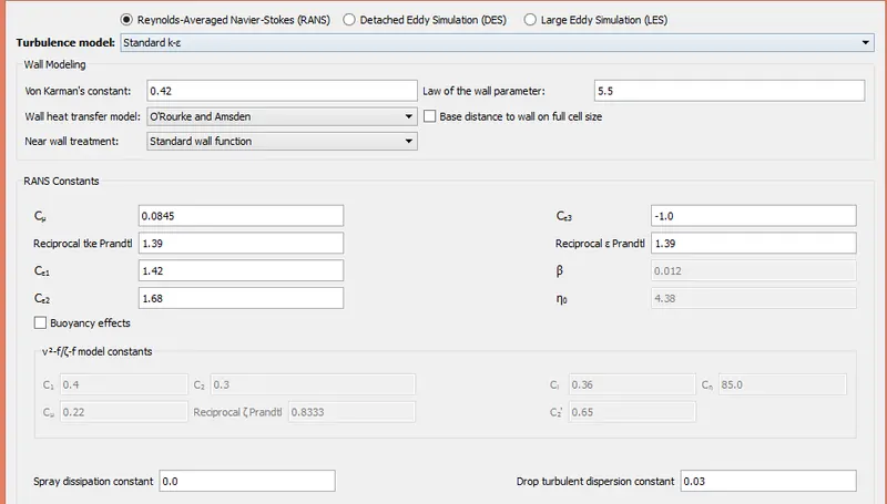
Turbulence Model: Standard K-e
Super Cycling:
Base Grid:
Enable Y+
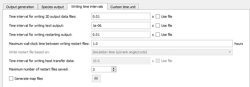
Output Files:
Grid Independence test:
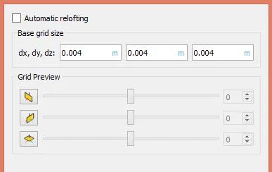
Case 1: grid size is 0.004m
Case 2: gird size is 0.003m
Case 3: gird size is 0.002m
Case 1: grid size is 0.004m
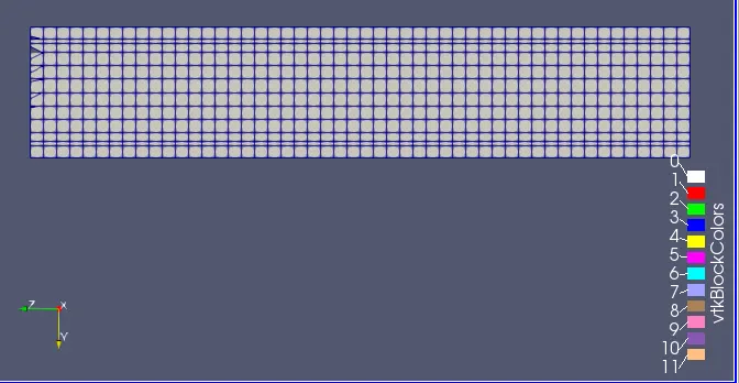
Mesh:
Contours:
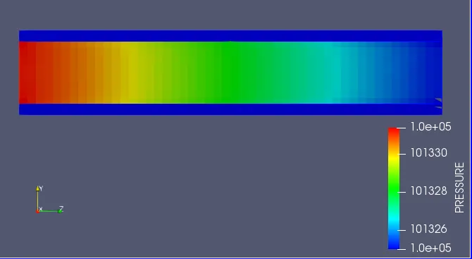
Pressure:
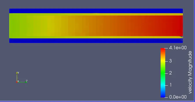
Velocity:
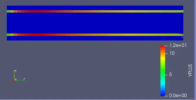
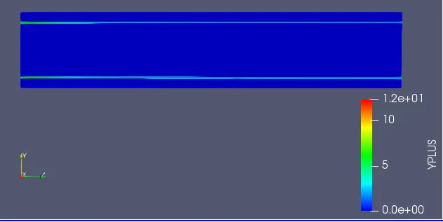
Y+:
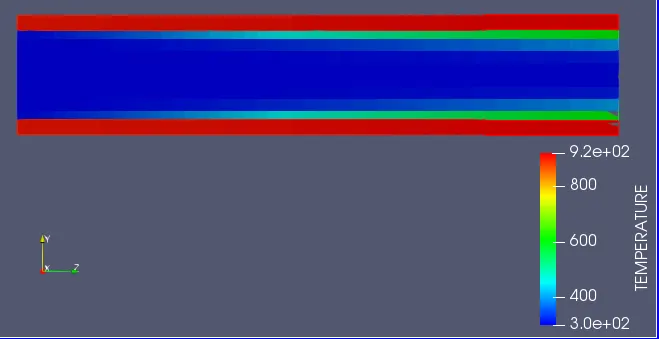
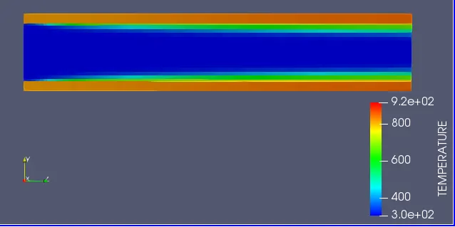
Temperature:
Animation link:
https://youtu.be/MuLOxcMBMqc
Plots:
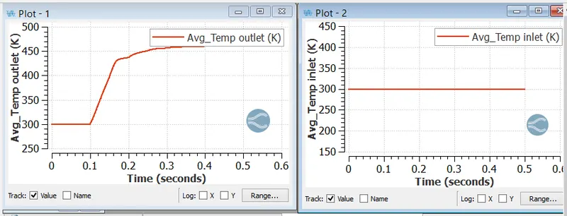
Temperature at inlet and outlet:
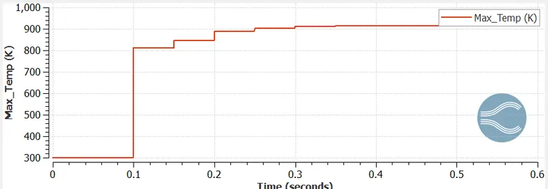
Temperature at Solid region:
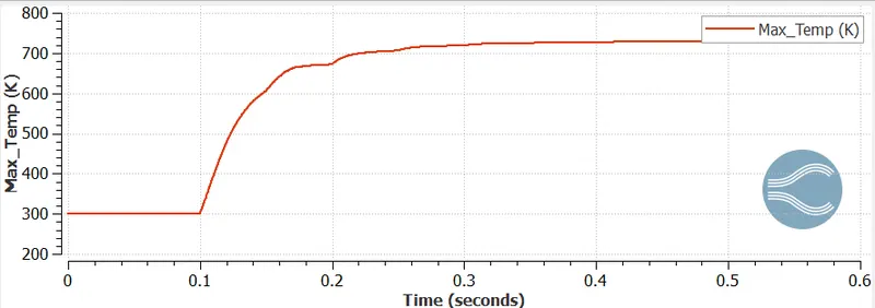
Temperature at fluid region:
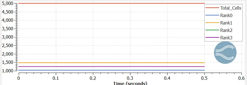
Total cell count:
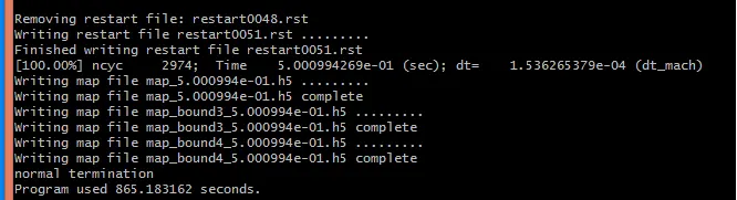
Calculation time:
Observations:
The total number of cells for this simulation is 5000
The max temperature of the solid region is 915K
The max temperature of the fluid region is 728K
The Average temperature at outlet of the pipe is 460K
The Average temperature at inlet of the pipe is 300K
The total simulation time is 865 sec.
Case 2 : gird size is 0.003m
Mesh:
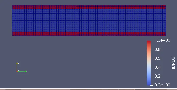
Contours:
Pressure:
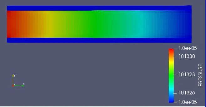
Velocity:
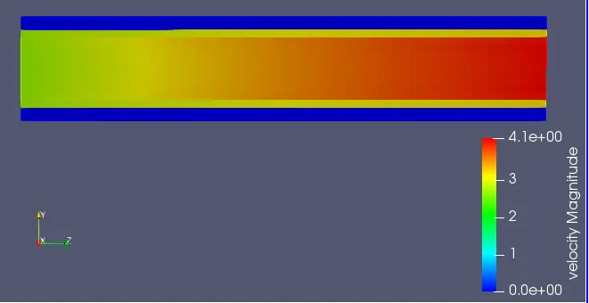
Y+ :
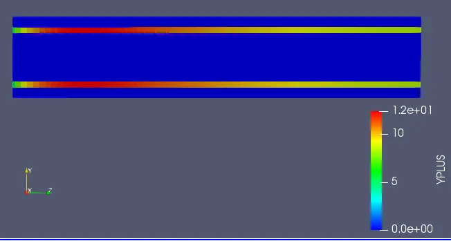
Temperature:
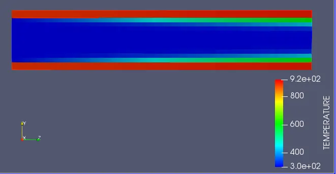
Animation Link:
https://youtu.be/5Nqw2ucmJK0
Plots:
Temperature at inlet and outlet:
Temperature at Solid region:
Temperature at fluid region:
Total cell count:
Calculation time:
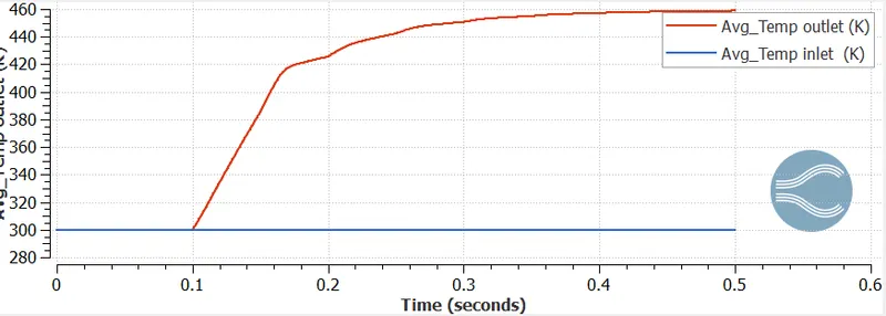
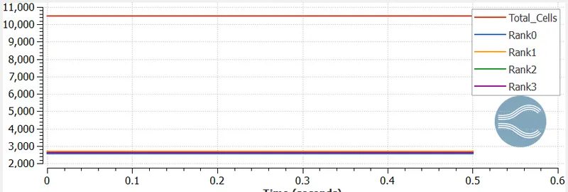
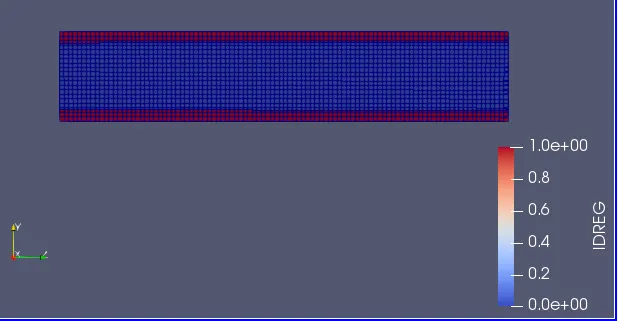
The total number of cells for this simulation is 10496
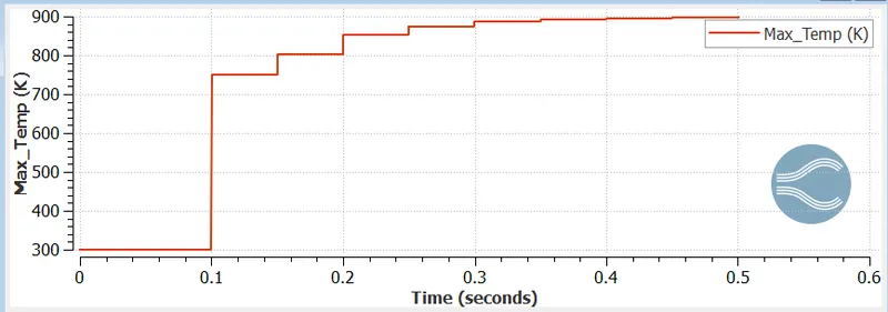
The max temperature of the solid region is 897K
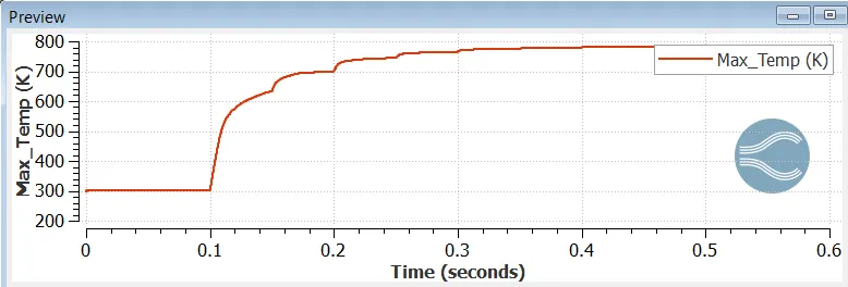
The max temperature of the fluid region is 783K
The Average temperature at outlet of the pipe is 458.9K
The Average temperature at inlet of the pipe is 300K
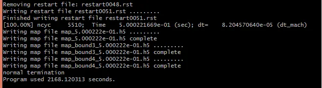
The total simulation time is 2168.12 sec.
3. Case 3: gird size is 0.002m
Mesh:
Contour:
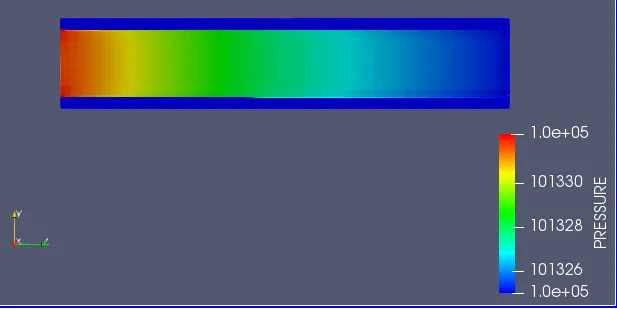
Pressure:
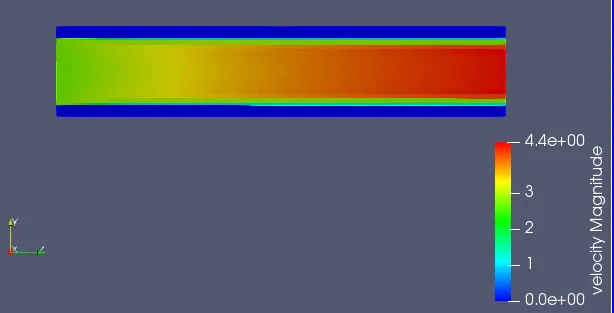
Velocity:
Y+:
Temperature:
Animation link:
https://youtu.be/kAMGkrVk8lg
Plots:
Temperature at inlet and outlet:
Temperature at Solid region:
Temperature at fluid region:
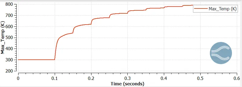
Total cell count:
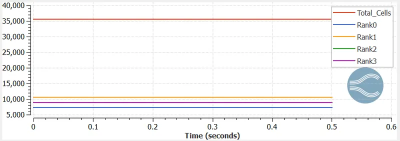
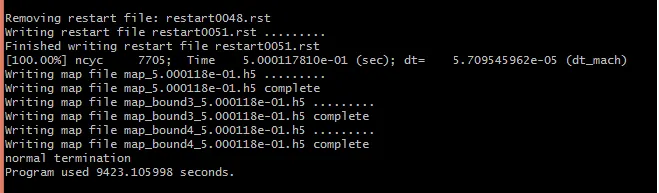
Calculation time:
The total number of cells for this simulation is 35600
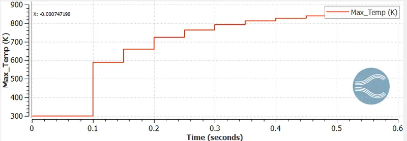
The max temperature of the solid region is 846.25K
The max temperature of the fluid region is 789.54K
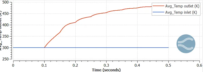
The Average temperature at outlet of the pipe is 485.15K
The Average temperature at inlet of the pipe is 300K
The total simulation time is 9423.105 sec.
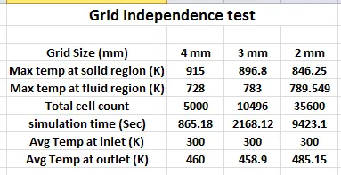
Grid Independence test:
Observations:
If Increase the mesh refinement, total number of cells increases and simulation time also increases.
Maximum temperature at solid region is decreasing when increase mesh refinement.
Maximum temperature at fluid region is increases when increases mesh refinement.
Average temperature at outlet also increases when mesh refinement.
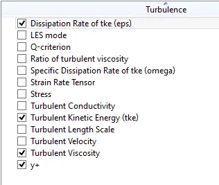
The Maximum Y+ value is seen in first and second case is 12, for the third case Y+ value is 8 only.
Second one is given the good results as compared to simulation time and temperature effects.
Y+:
The Y+ value is a dimensionless parameter used to determine which wall function has to used, in order to predict the nature and behaviour of the fluid near the wall.
Therefore it is less than 10; it is in viscous sub-layer, if it is more than 30, it is in turbulent. If it is in between then it is transition.
The first and second case Y+ value is 12, which means it is in transition phase. This value has minor significance for CHT Simulation.
For the third case Y+ value is 8, which means it is in visocous-sub layer region.
Effect of super cycle stage interval
1. Super cycle stage interval 0.04
2. super cyle stage interval to 0.03
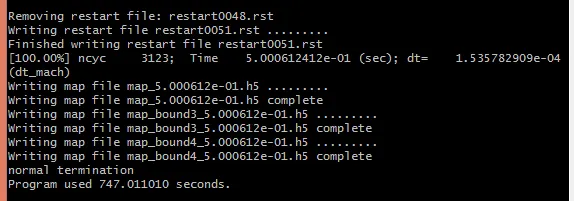
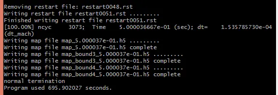
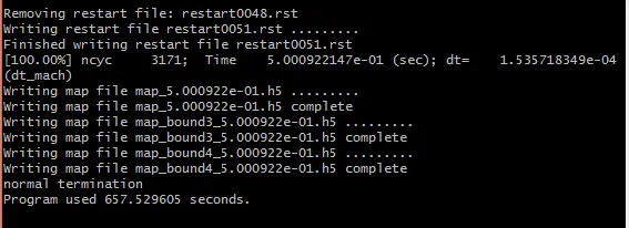
simulation time:
3. super cyle stage interval to 0.02
4. supercyle stage interval to 0.01
Plots:
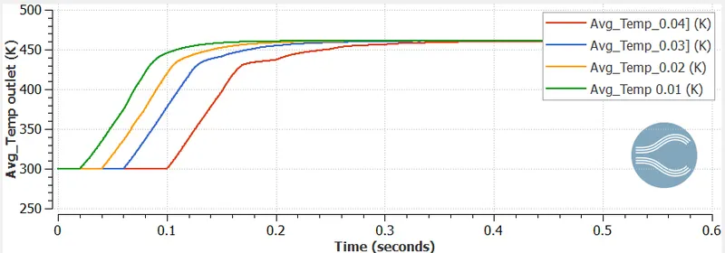
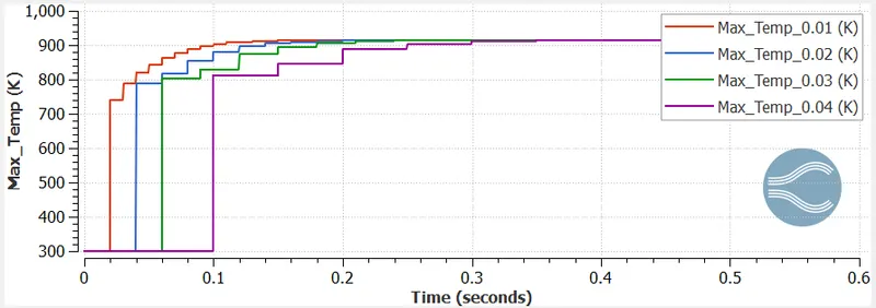
Temperature at outlet:
Observations:
The above plots show how the simulation proceeds, when the super cycling stage interval is varied.
As the stage interval reduced, the solution converge faster and reaches the steady state.
All the cases the final temperature values are same.
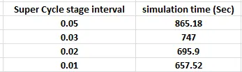
Effect of Super cycling:
Observations:
The above shows the Simulation time varies with respect to the super cycle stage interval is shown.
As Stage interval is increases, simulation time also increases. Because the time take to attain steady state.