Week 7: Shock tube simulation project
Aim:
- Setup a transient shock tube simulation
- Plot the pressure and temperature history in the entire domain - Explain the result
- Plot the cell count as a function of time - Explain the result
Software Used : Converge CFD
Theory:
Shock tubes are devices for studying the flow of high-temperature and high-velocity compressible gas.
A high-temperature supersonic gas flow is initiated in a shock tube as a result of rupture of a diaphragm separating two gases in high-pressure and low-pressure chambers. An unsteady rarefaction wave passes into the "driver" gas in the high-pressure chamber with a velocity a few kilometers per second. This results in the drivers gas flowing into the low pressure gas, pushing the gas in the low pressure chamber ahead of it. The shock wave propagates in the low-pressure chamber ahead of this flow of the studied gas. The velocity of the driven gas flow is equal to that of the driver gas flow. The wave (x − t) pattern, the schematic of the shock tube, and distribution of pressures p and temperatures T along the tube axis are presented in Figure 1. The parameters are denoted by 0 in the low-pressure chamber of the shock tube, 1 behind the incident shock wave, 2 behind the contact surface, 3 in the rarefaction wave, 4 in the high-pressure chamber, and 5 behind the reflected wave. In order to generate a shock wave with the specified pressure ratio p1/p0 in a shock tube, it is necessary to provide the pressure ratio p4/p0 over the shock tube diaphragm, which satisfies the relation
where a is the velocity of sound, γ the adiabatic exponent, u1 the velocity of gas flow behind the shock wave producing the pressure ratio p1/p0. Varying the length of high- and low-pressure chambers, we can find a regime of shock tube operation under which the shock wave reflected from an end meets the tail of the rarefaction wave and the head of the reflected rarefaction wave at a fixed point. This regime known as the "joined" contact surface regime ensures the maximum time of undisturbed state behind the reflected wave. The maximum flow parameters achieved in shock tubes depend on the design of the high-pressure chamber. According to this, shock tubes can be devided into four groups.
(1) Shock tubes with an inert gas in the high-pressure chamber. In this case a driver gas is hydrogen or helium at a pressure ranging from several to a hundred atmospheres and of ambient initial temperature. For pressures in the low-pressure chamber from 1 to 100 mmHg, the shock wave velocities range from 0.5 to 6 km/s. The temperature behind the shock wave is from 1000 to 10,000 K. The length of the high pressure gas zone, depending on the tube length and the shock wave velocity, is from several centimeters in laboratory tubes, whose length does not exceed 10 meters, to a meter in test shock tubes 50 to 100 meters long.
(2) Shock tubes with an explosive in the high-pressure chamber. In this case, in the high-pressure chamber, a hydrogen-oxygen-helium mixture or a solid explosive charge are used to increase the initial temperature of a driver gas. The gas temperature behind the shock wave amounts to 20,000 K in an inert gas and 15,000 K in a dissociating gas.
(3) Electrically driven shock tubes. These are tubes in which a discharge chamber with discharge-heated gas is used instead of the high-pressure chamber. Electrically driven shock tubes are designed with and without diaphragms because the parameters of the driver gas increase sharply as a result of discharge. In these shock tubes the velocity of the shock waves varies from 10 km/sec at initial pressures of several millimeters Hg to 100 km/sec at initial pressures fractions of a millimeter Hg. Gas temperature reaches a few tens of thousands of degrees.

Geometry Creation:
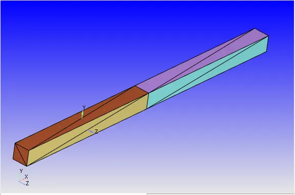
Dimensions:
The length of the tube is 0.2m
width and height of the tube is 0.01m and 0.01m respectively.
Before going to case setup, check any boundary flaging error in the geometry with help of Diagnosis.
Diagnosis:
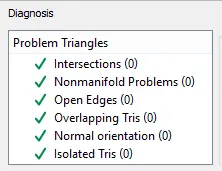
The diagnosis is performed, there are no errors in the geometry.
Case setup:
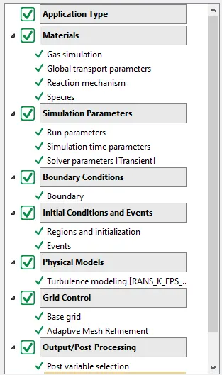
Application type: Time based simulation
Materials: Air
Species: N2 and O2
Simulation Parameters:
Solver: Transient simulation, Density based
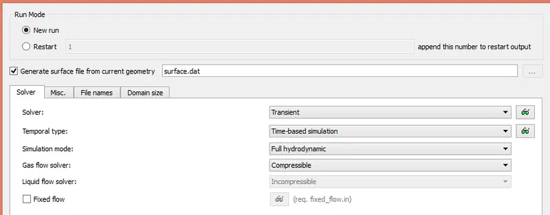
Simulation time parameters:
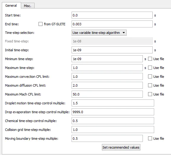
Solver Parameters:

Boundary Conditions:
High Pressure region ( N2, 6 bar, 300K)
Low pressure region ( O2, 101325ka, 300K)
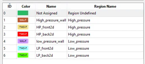
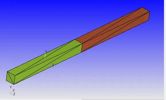
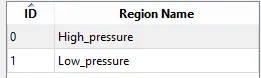
Two regions are created in the intial conditions
Events:
0-0.001s close
0.001s-0.003s open

Physical model:
Turbulence (RANS-K-e)
Grid Control:
Base grid : 1mm
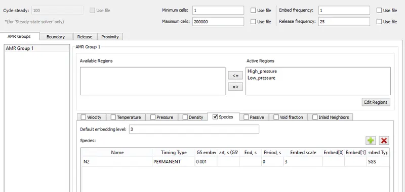
Adaptive mesh Refinement: N2 species, SGS- 0.001
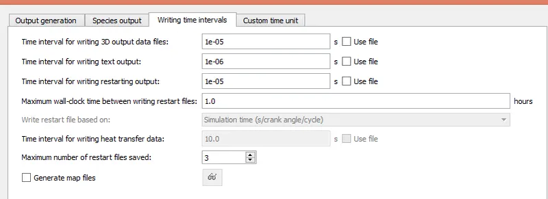
Output files:
Mesh:
A base grid of 0.001m is used along all the directions.
Adaptive mesh refinemet is concerned, the sub grid scale criterion of 0.001 for 3 embedded layers are used for N2 species.
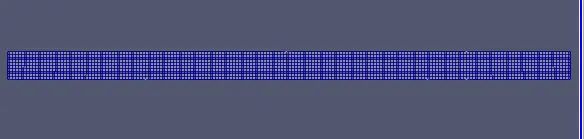

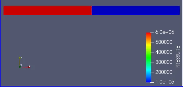
The lift side is high pressure and right side is low pressure region.
Contours:
Pressure:
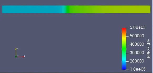
Animation Link:
Temperature:
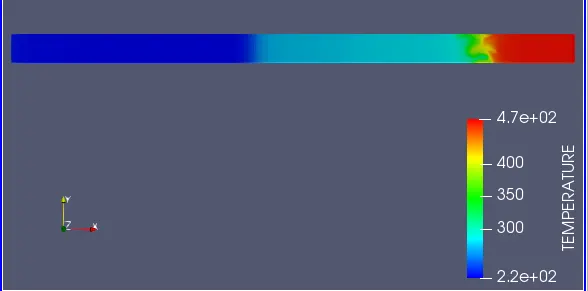
Animation Link:
Velocity:
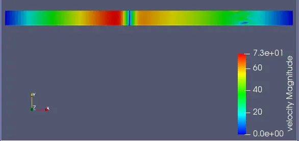
Animation link:
Plots:
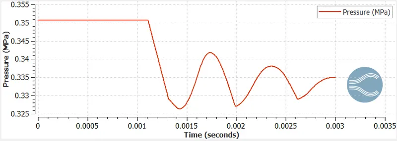
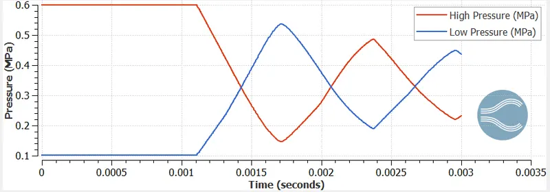
Pressure:
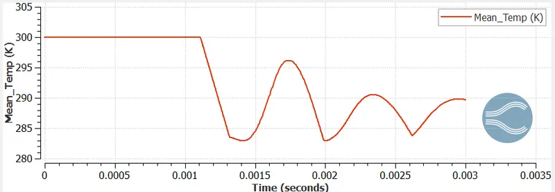
Temperature:
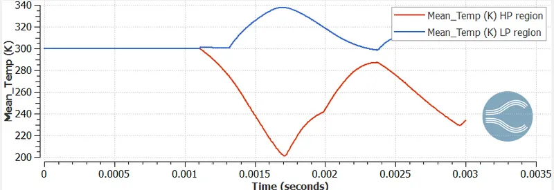
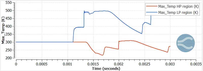
Total cell count:
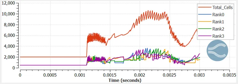
The cell count is rapidly changing because we are using the Adaptive mesh refinement on the basis of the N2 species
After opening the diaphram the shock wave is produced which gives th suddden accleration in the medium.
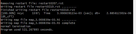
Simulation time:
Observations:
The process of generation of shock and expansion waves continues till the pressure difference in the domain out.
AMR keeps on refining the mesh in the wavefront untill the rate of change of concentration of N2 is below the SGS value.
The diaphram breaks at 0.001s, the pressure in the high region reduces and increases the pressure in the low region.
Sudden increase in the pressure in the low region causes the shock and expansion due to decrease the pressure in higher region.
Shock wave increases the temperature and expansion wave decreases the temperature.
A sinusoidal behaviour is observed in the pressure plots.
Shock waves are reflected when the gases in the low pressure region are compressed.