Week 3.5 - Deriving 4th order approximation of a 2nd order derivative using Taylor Table method
Aim: Deriving 4th order approximation of a 2nd order derivative using Taylor Table method of the function exp(x)*cos(x) and compare it with the 3 numerical approximations
Software Used: MATLAB
Formulation for the Taylor table mthods for Central difference Scheme.
f''(x) = af(x-2h) + bf(x-h) + cf(x) +df(x+h) + ef(x+2h)/(h^2)
Formulation for the Taylor table mthods for Left skewed Scheme.
f''(x) = af(x) + bf(x-h) + cf(x-2h) +df(x-3h) + ef(x-4h)/(h^2)
Formulation for the Taylor table mthods for Right skewed Scheme.
f''(x) = af(x) + bf(x+h) + cf(x+2h) +df(x+3h) + ef(x+4h)/(h^2)
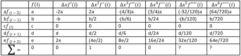
Forth order Centred Scheme:
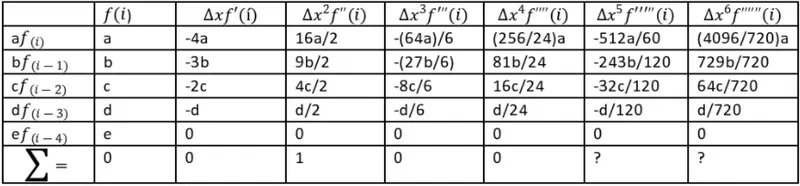
Forth order left skewed Scheme:
Forth order Right skewed Scheme:
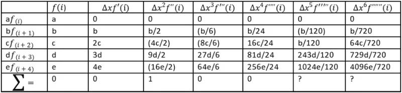
The Taylor's table is made by expanding the well known Taylor's series.
In the above equations we need to find the coefficients a,b,c,d and e. For each scheme by comparing the coefficients of Taylor’s series expansion.
Fourth order Central difference scheme coefficients
a = -0.0833, b= 1.333, c = -2.5, d = 1.333, e = -0.8333
Fourth order left sided skewed scheme coefficients
a = 0.91667, b = -4.667, c =9.5, d = -8.667, e = 2.9167
Fourth order Right sided skewed scheme
a = 2.91667, b = -8.6667, c = 9.5, d =-4.667, e = 0.91667
Matlab Code:
Function code for Central difference scheme:
function err_centraldiff = central_diff_scheme_4th_order(x,dx)
% Analytical function = exp(x)*cos(x)
% f''(x) = -2*sin(x)*exp(x)
analytical_derivative = -2*sin(x)*exp(x);
% numerical derivative
central_diff = ((-0.0833*cos(x-2*dx)*exp(x-2*dx))+ (1.3333*cos(x-dx)*exp(x-dx))+(-2.5*cos(x)*exp(x))+(1.333*cos(x+dx)*exp(x+dx))+(-0.0833*cos(x+2*dx)*exp(x+2*dx)))/(dx^2)
err_centraldiff = abs(analytical_derivative - central_diff)
end
Function code for Left-Skewed scheme:
function err_leftskewed = left_skewed_4th_order(x,dx)
% Analytical function = exp(x)*cos(x)
% f''(x) = -2*sin(x)*exp(x)
analytical_derivative = -2*sin(x)*exp(x);
% numerical derivative
left_skewed = ((0.91667*cos(x)*exp(x))+ (-4.667*cos(x-dx)*exp(x-dx))+(9.5*cos(x-2*dx)*exp(x-2*dx))+(-8.667*cos(x-3*dx)*exp(x-3*dx))+(2.9167*cos(x-4*dx)*exp(x-4*dx)))/(dx^2)
err_leftskewed = abs(analytical_derivative - left_skewed)
end
Function code for Right-Skewed scheme:
function err_rightskewed = right_skewed_4th_order(x,dx)
% Analytical function = exp(x)*cos(x)
% f''(x) = -2*sin(x)*exp(x)
analytical_derivative = -2*sin(x)*exp(x);
% numerical derivative
right_skewed = ((2.9167*cos(x)*exp(x))+ (-8.667*cos(x+dx)*exp(x+dx))+(9.5*cos(x+2*dx)*exp(x+2*dx))+(-4.667*cos(x+3*dx)*exp(x+3*dx))+(0.91667*cos(x+4*dx)*exp(x+4*dx)))/(dx^2)
err_rightskewed = abs(analytical_derivative - right_skewed)
end
Main Program:
clear all
close all
clc
x = 2*pi;
dx = linspace(pi/3,pi/3000,200);
% Analytical function = exp(x)*cos(x)
% f''(x) = -2*sin(x)*exp(x)
% Error of numerical derivative
for i = 1:length(dx)
% central difference approximation
error_central(i) = central_diff_scheme_4th_order(x,dx(i))
% second order approximation
error_right(i) = right_skewed_4th_order(x,dx(i))
% fourth order approximation
error_left(i) = left_skewed_4th_order(x,dx(i))
end
% plotting
loglog(dx,error_central)
hold on
loglog(dx,error_right)
hold on
loglog(dx,error_left)
legend('Central Difference','Right Skewed','Left Skewed')
xlabel('dx')
ylabel('error')
title('Fourth order Appoximation')
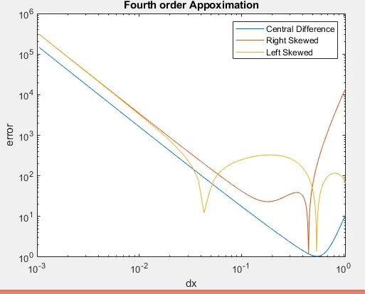
Plot:
Conclusion:
As seen the above plot, The central differencing scheme has very less error compared to other schemes.
When we don't have any nodes at the boundary then Skewed schemes are useful to approximate to improve the accuracy but when we have internal nodes available then centred ones are good.