Conjugate Heat Transfer Analysis on a graphics card.

Aim: Perform a steady-state conjugate heat transfer analysis on a model of a graphics card. 

Software Used: Ansys Fluent

Theory: 

Conjugate heat transfer: The Conjugate Heat Transfer (CHT) analysis type allows for the simulation of heat transfer between solid and fluid domains by exchanging thermal energy at the interfaces between them. Typical applications of this analysis type exist as, but are not limited to, the simulation of heat exchangers, cooling of electronic equipment, and general-purpose cooling and heating systems.

Conjugate heat transfer corresponds with the combination of heat transfer in solids and heat transfer in fluids. In solids, conduction often dominates whereas in fluids, convection usually dominates. Conjugate heat transfer is observed in many situations. For example, heat sinks are optimized to combine heat transfer by conduction in the heat sink with the convection in the surrounding fluid.

Heat Transfer by Solids and Fluids

Heat Transfer in a Solid

In most cases, heat transfer in solids, if only due to conduction, is described by Fourier’s law defining the conductive heat flux, q, proportional to the temperature gradient: .

For a time-dependent problem, the temperature field in an immobile solid verifies the following form of the heat equation:

Heat Transfer in a Fluid

Due to the fluid motion, three contributions to the heat equation are included:

1. The transport of fluid implies energy transport too, which appears in the heat equation as the convective contribution. Depending on the thermal properties on the fluid and on the flow regime, either the convective or the conductive heat transfer can dominate.
2. The viscous effects of the fluid flow produce fluid heating. This term is often neglected, nevertheless, its contribution is noticeable for fast flow in viscous fluids.
3. As soon as a fluid density is temperature-dependent, a pressure work term contributes to the heat equation. This accounts for the well-known effect that, for example, compressing air produces heat.

Accounting for these contributions, in addition to conduction, results in the following transient heat equation for the temperature field in a fluid:

 Geometry:

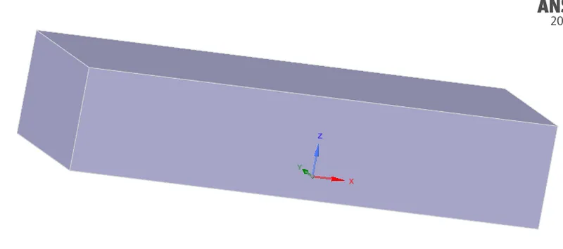
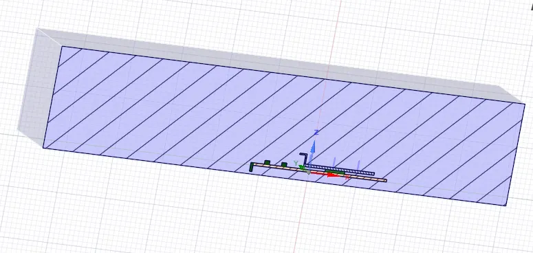
Import the step file in Ansys Space claim. next create the Enclosure for the model.

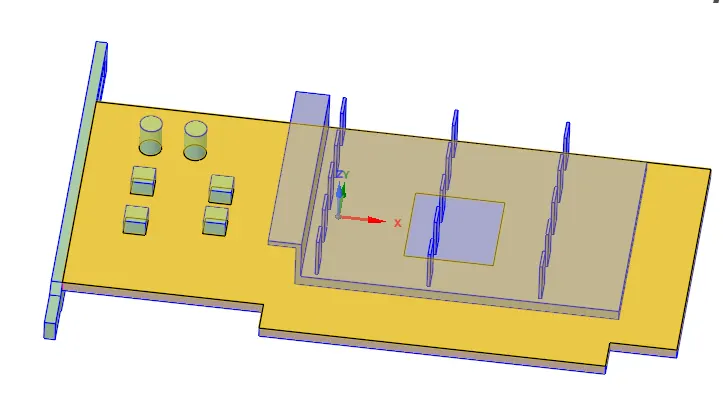
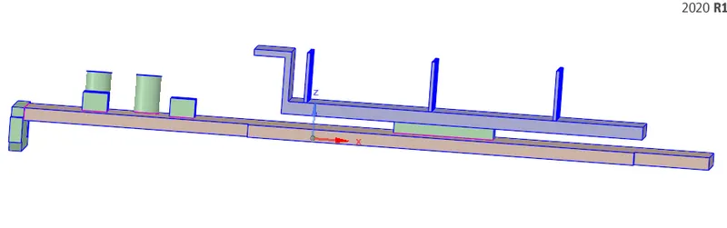
Enable Share topology option for conformal mesh. otherwise mesh will be failed

Mesh:

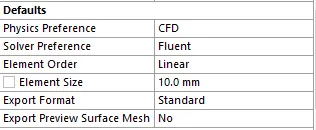
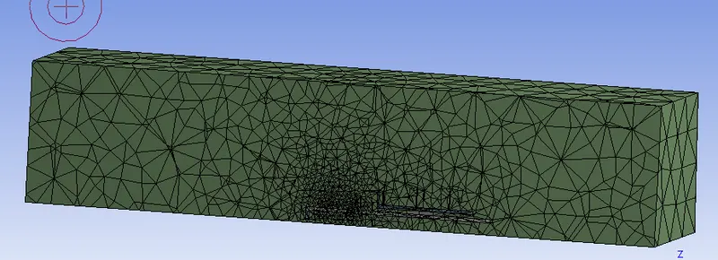
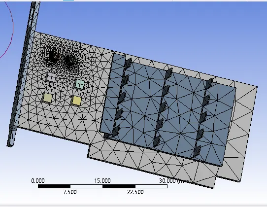
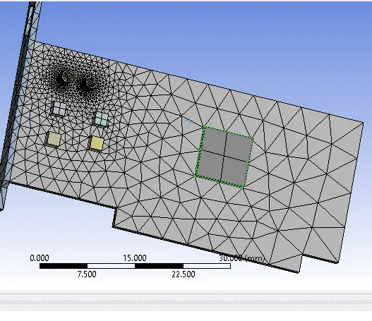
Base line Mesh:

   

Conformal Mesh:

  

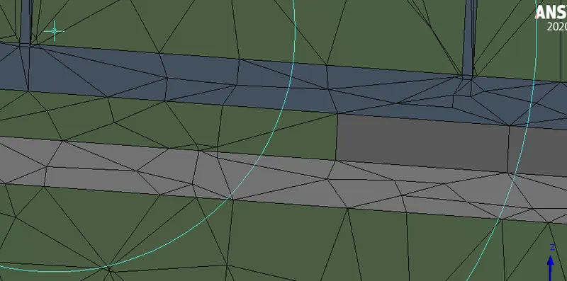
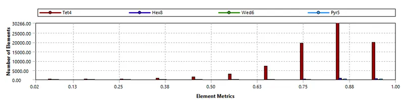
Mesh Matrix:

Case Setup:

Solver is Pressure based and Steady State simulation.

Enable the Energy equation for simulating the temperature behaviour.

The standard K-epsilon realizable turbulence model is used for CHT Analysis to solve the problem for getting converges faster.

Materials:

Fluid: Air

Solid: Steel, Silicon, copper

The model of this graphic card consists of 3 main components, namely Base,Processor and fins, each made up of materials like steel, silicon and copper respectively.

The Physical properties of the materials are given in below.

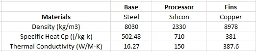
The Processor is located in between the base and fins as shown in the geometry.

The Processor produces the heat with its usage.

The base is used to support the assembly.

The Fins are used for cooling the processor which conducts heat. Fins are cooled by the air,(27 degree centigrade) passes over the graphic card assembly.

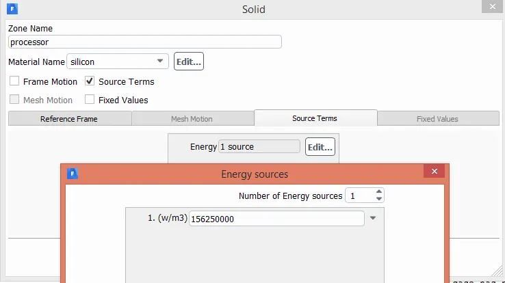
The Processor produces heat, so heat generation rate value are given the inputs. The calculation of heat generation rate by the processor is given by:

Volume of the processor as per the geometry = 0.064m3

Heat generation rate = power uses/volume of the processor

assuming power uses is 10W

So heat generation rate = 10*10e6/0.064

                                   = 1.5625e8 W/m3

Cell gone conditions: Processor

 Boundary Conditions:

The velocity of inlet air is 1 m/s and temperature is 300K.

The heat generation term is added to the processor in the cell conditions.

Initialization:

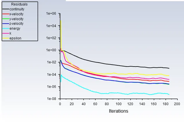
Initially the solution is run for 200 iterations and simulation is converges at 186 iterations.

Plots:

Residual plot:

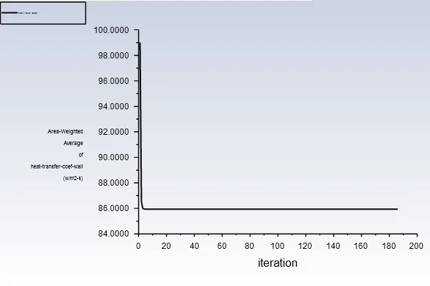
Heat transfer Coefficient:

Contours:

Temperature on processor:

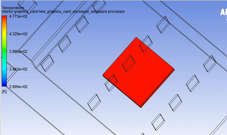
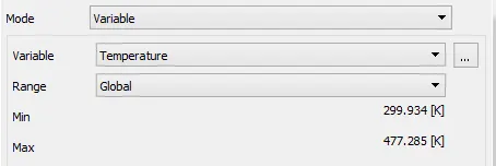
The Maximum temperature of the processor is 477.285 K

Heat transfer coefficient Processor:

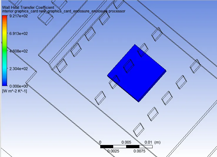
The Maximum heat transfer coefficient on the processor are 921.674 (w/m2k)

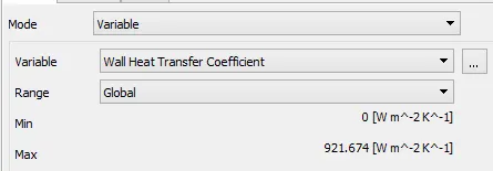
Temperature distribution on graphics card:

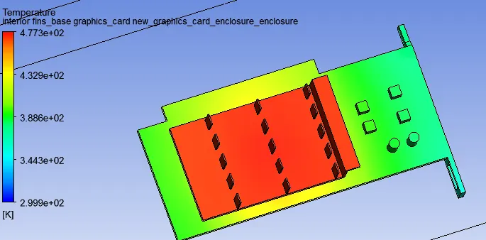
Heat transfer coefficient:

Temperature at plane:

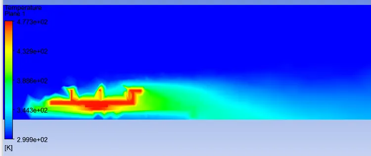
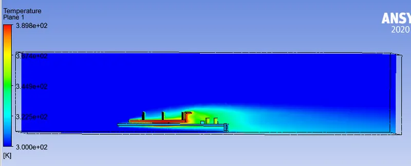
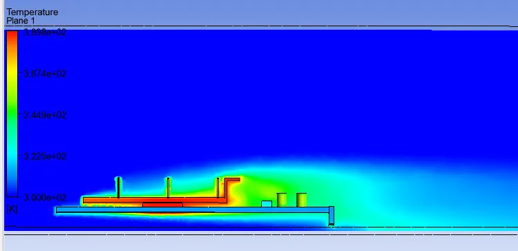
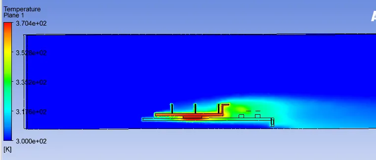
The temperature of air gradually increases as it passes over the graphic card assembly due to the convection. Where in heat is transferred from the solid to fluid.

Velocity at plane:

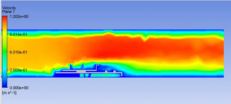
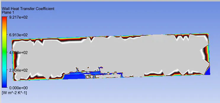
Heat transfer coefficient at plane:

Velocity vector:

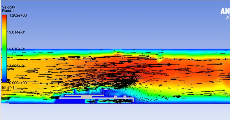
Hotspot 

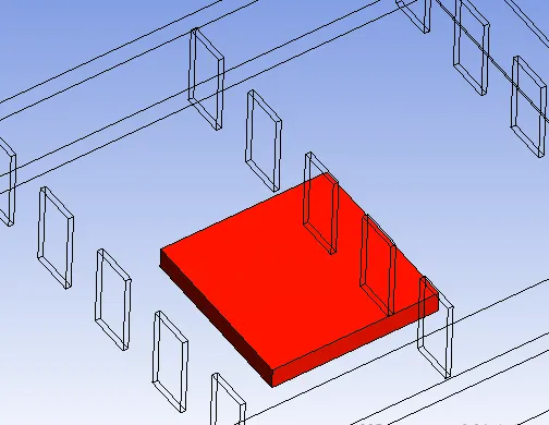
Temperature plot showing hot spot:

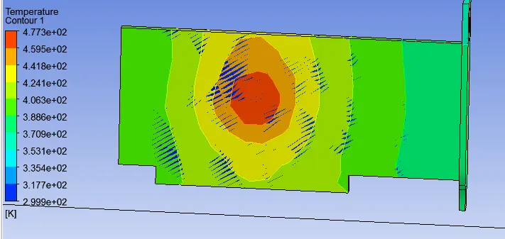
The potential hotspot in the graphic card is Processor, it is only heat generating part in the entire assembly.

The temperature of the remaining components in the assembly is influenced by the heat generated by the processor.

As work load increases, Processor produce a higher amount off heat.

Observations:

The highest temperature attained by the graphic card of this simulation is 477K.

We seen that temperature of the fins is comparatively higher than the base, because fins material having higher thermal conductivity than the base material.

The Application of fin is dissipate the heat, if the temp of the fins is high, the more heat can be dissipated.

We got desired results by running the simulations using the baseline mesh.

Now we can run the same simulations at different velocities using the refined mesh.

The solution converges at 186 iterations only

Refined Mesh:

To generate the refined mesh, the mesh element size was reduced. Separate mesh element sizing is provided for the solid and fluid domain. The mesh element size for solid and fluid domain is 0.9mm.

A total number of nodes is 83279 and 481203 elements were created. Share topology feature was enabled in space claim for conformal mesh.

  

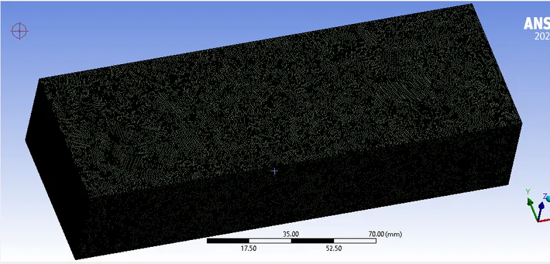
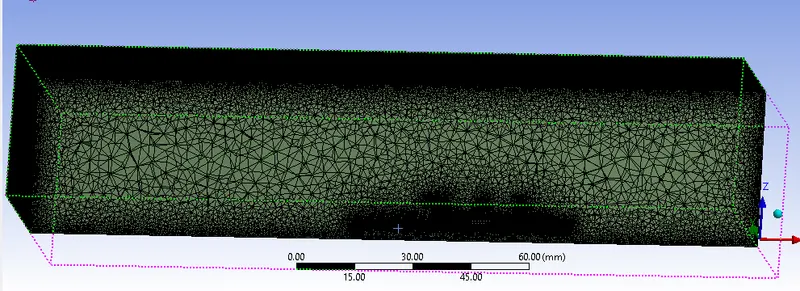
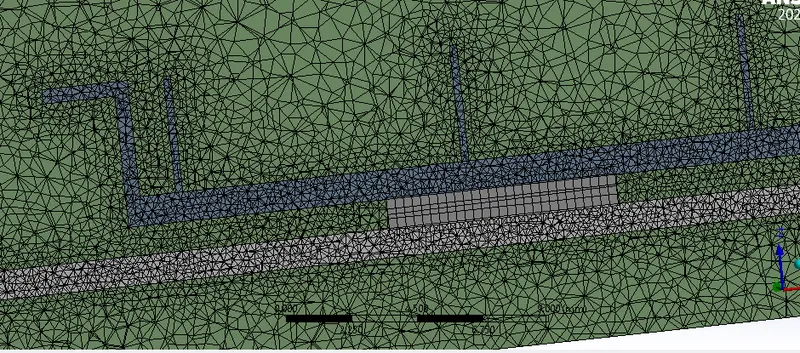
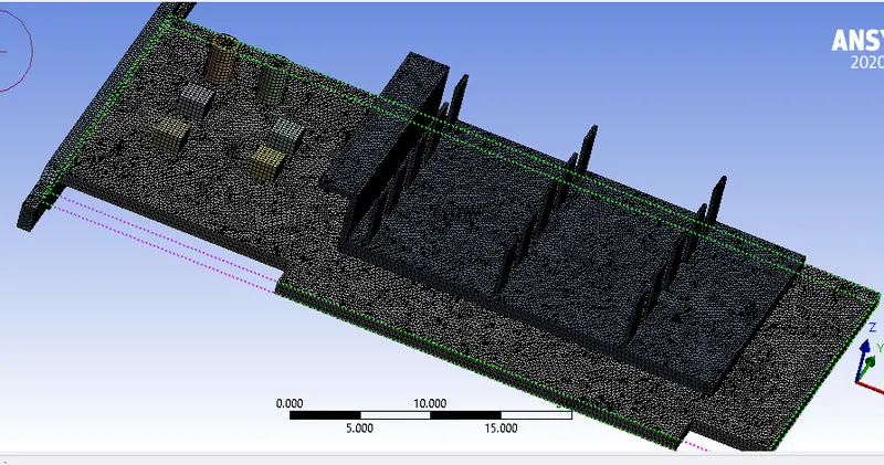
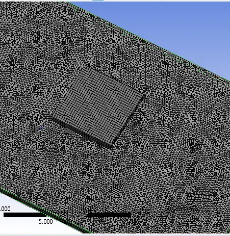
Majority of the mesh elements have mesh quality greater than 50% , this mesh is said to be suitable to perform CHT Analysis.

Case Setup:

Same as the baseline conditions

Plots:

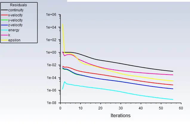
Residual Plots:

Heat transfer coefficient:

Contours:

Temperature on processor:

Heat transfer coefficient Processor:

Temperature distribution on graphics card:

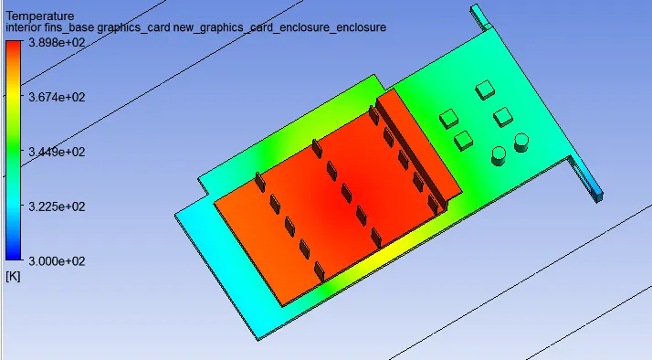
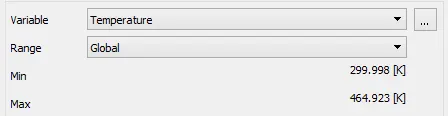
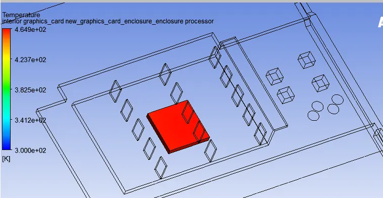
The highest temperature attained by this condition is 464.923 K.

We see that temperature of the fins is comparatively higher than that to the base. Because the copper material used for the fins having greater thermal conductivity.

Fins are dissipating the more heat.

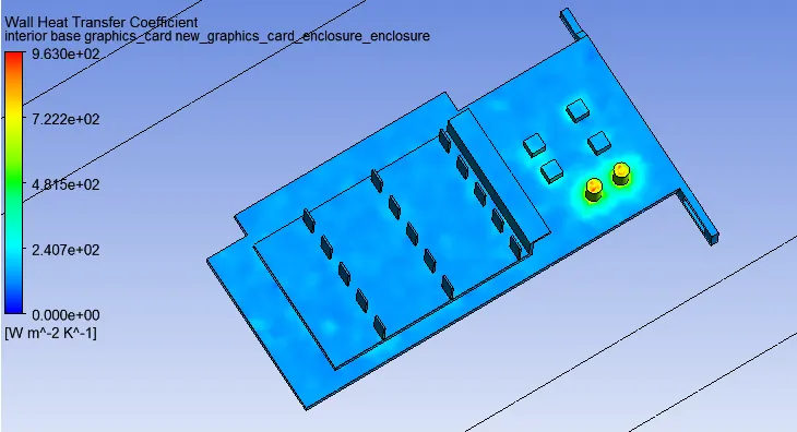
Heat transfer coefficient:

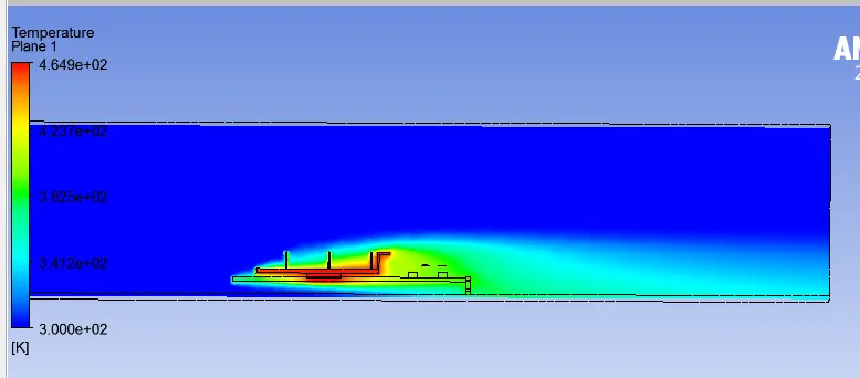
Temperature at plane:

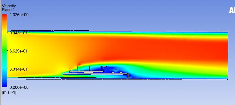
Velocity at plane:

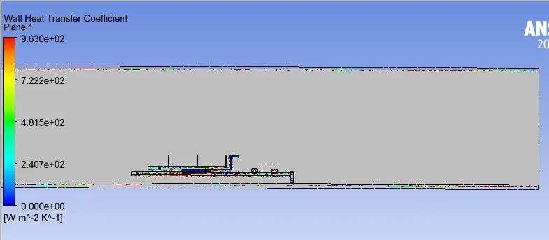
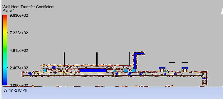
Heat transfer coefficient at plane:

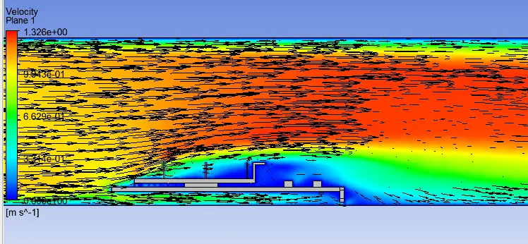
Velocity vector:

Hotspot:

 

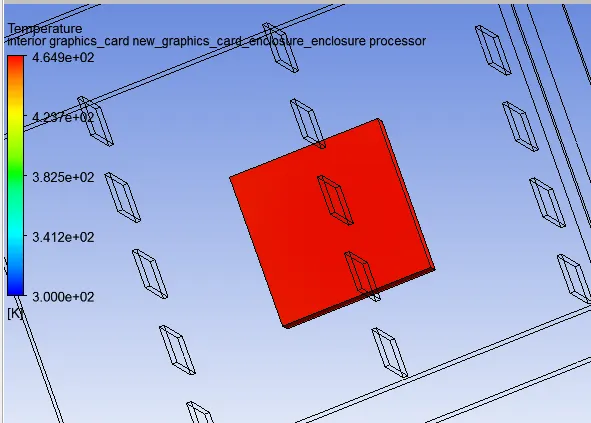
Temperature plot showing hot spot:

 

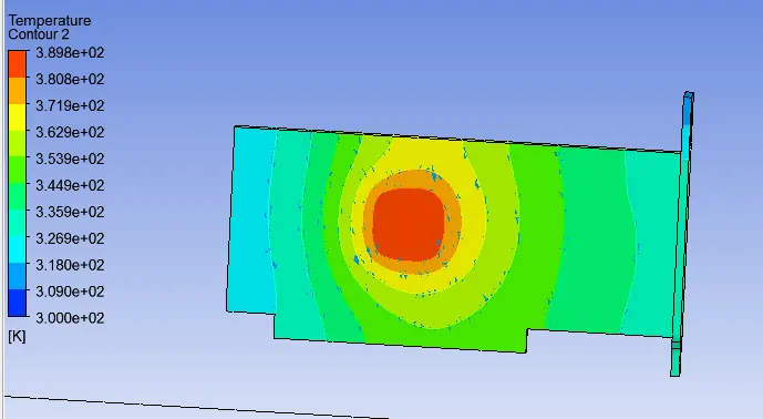
Observations:

The hotspot in the graphic card is processor which is direct contact to the base in the assembly. The above graph shows the how hotspot are formed in the base region.

The temperature from the inlet remains constant. The temperature of air increases as it passes over the entire assembly from the solid to the fluid. 

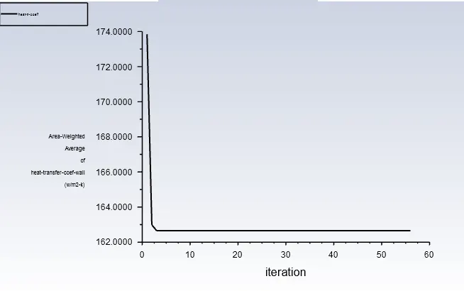
The mesh refinement is done in this condition  and the solution is converges at 56 iterations.

Increase the mesh refinement solution converges faster with compare to base line condition.

Refined Mesh Velocity at 3 m/s :

Residual plot:

Heat transfer coefficient:

Contours:

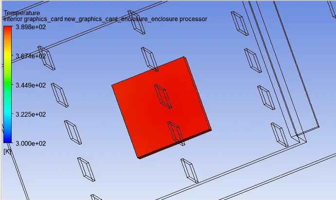
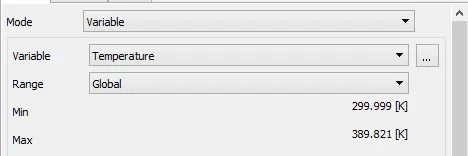
Temperature on processor:

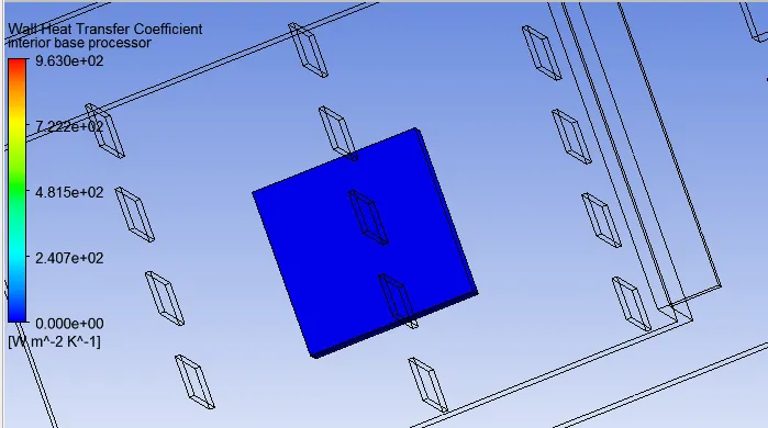
Heat transfer coefficient Processor:

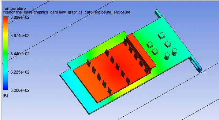
Temperature distribution on graphics card:

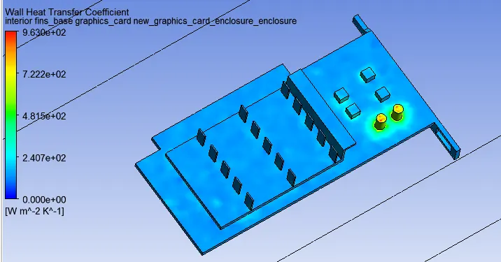
Heat Transfer Coefficent:

Temperature at plane:

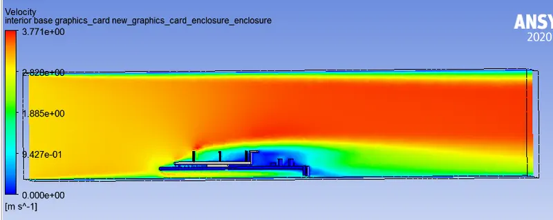
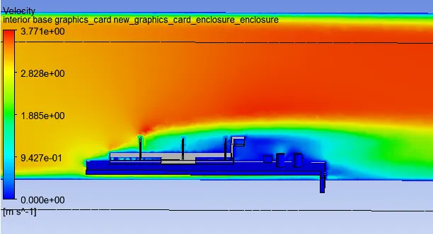
Velocity at plane:

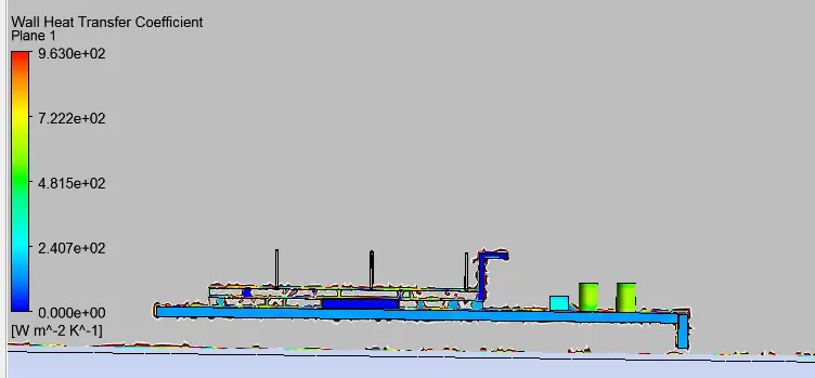
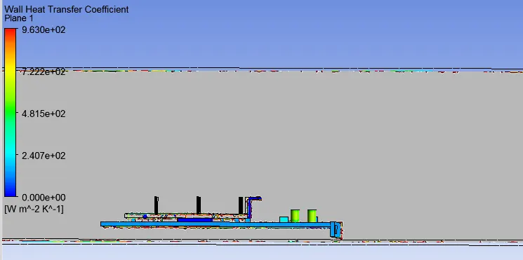
Heat transfer coefficient at plane:

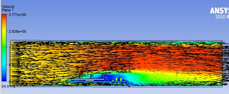
Velocity vector:

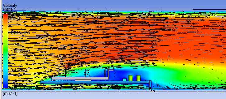
Hotspot:

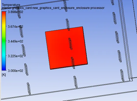
Temperature plot showing hot spot:

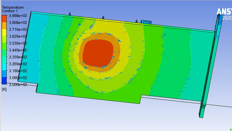
The hotspot in the graphic card is processor which is direct contact to the base in the assembly. The above graph shows the how hotspot are formed in the base region.

Observations:

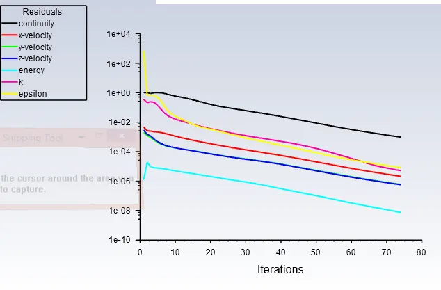
The solution is converges for this condition is 74 iterations.

Increases the velocity at inlet, solution for convergence takes more time.

The maximum temperature of the processor for this condition is attaining 389K.

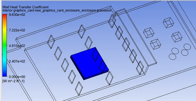
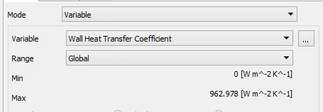
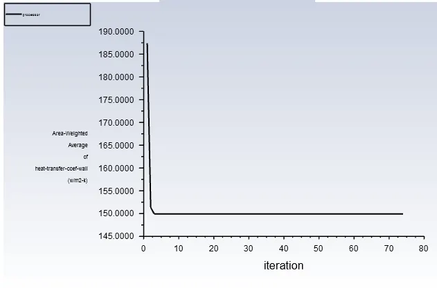
The Maximum heat transfer coefficient is attaining for this condition is 962.978 W/m2k.

Velocity at 5m/s:

Plots:

Residual Plots:

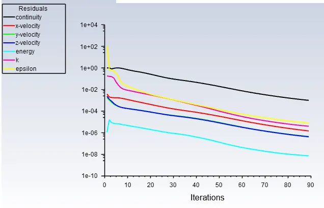
Heat transfer coefficent:

Contour:

Temperature at processor:

Heat transfer coefficient Processor:

 

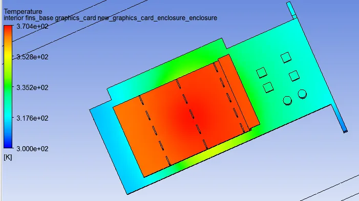
Temperature contour:

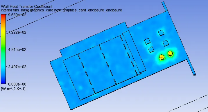
Heat transfer Coefficent:

Temperature at plane:

 

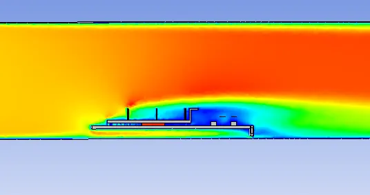
Velocity at Plane:

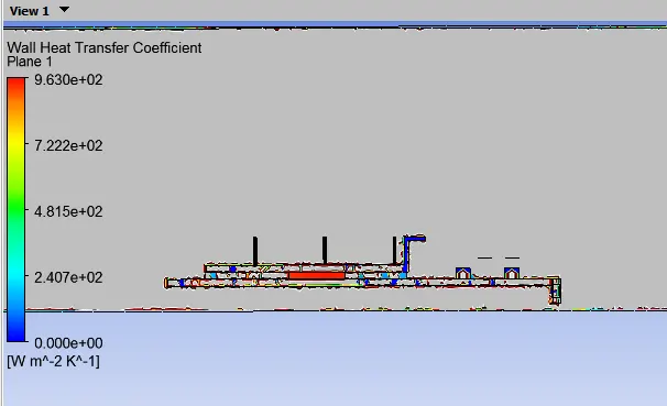
Heat transfer coefficent:

Temperature plot showing hot spot:

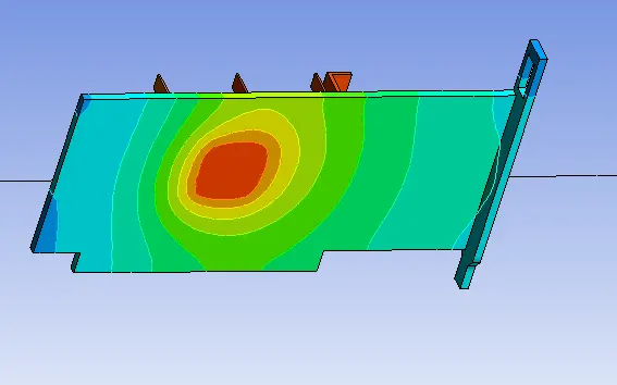
The hotspot in the graphic card is processor which is direct contact to the base in the assembly. The above graph shows the how hotspot are formed in the base region.

Observations:

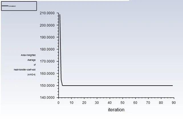
The solution is converges for this condition is 90 iterations.

Increases the velocity at inlet, solution for convergence takes more time.

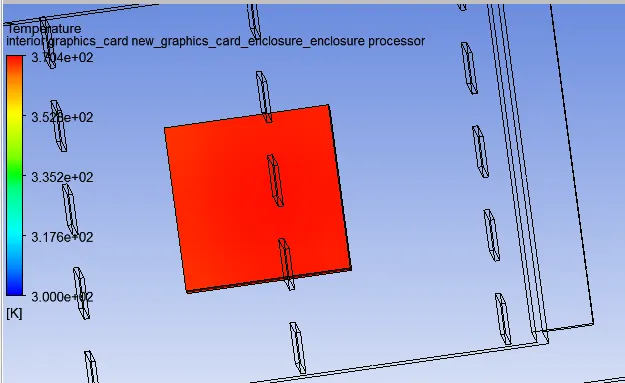
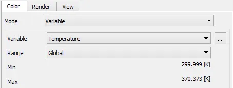
The maximum temperature of the processor for this condition is attaining 370.373K.

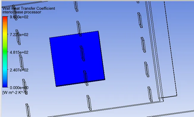
The Maximum heat transfer coefficient is attaining for this condition is 962.978 W/m2k.

We observed that increases in the velocity, convergence time increases in the problem.

The maximum temperature at processor is reduced slightly for increases the velocity because of velocity of flow is increased, more amount of heat is carried away by air.

Heat transfer coefficent is contact for all conditions.

Heat transfer coefficent is the highest in the regions which are contact with the processor. This region is not affected by change in the flow velocity since there is no air flow present.

From the above table, refined mesh gives more accurate results compared to the coarse mesh.

With increase in velocity, Temperature and region of hotspot generated on solid base of processor is reduced.