Challenge on Combustion
Aim: To perform combustion simulation on the combustor model and plot the variation of the mass fraction of the different species.
To plot contours and line plots for CO2, H2O, CH4, N2, O2, NOx emissions & Soot formation.
To add the water content in the fuel 5% to 30% by mode and observe the effect of it on the results.
Software used: Ansys Fluent
Theory:
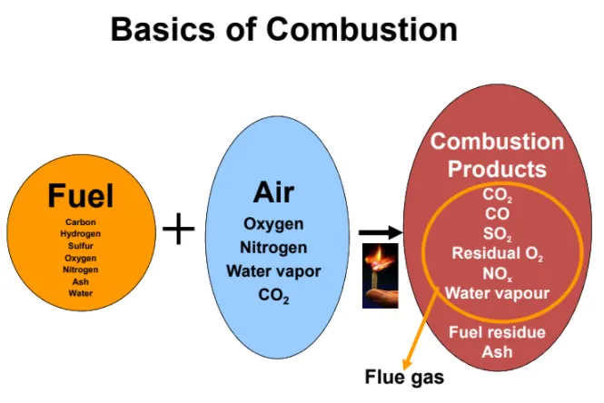
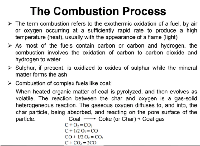
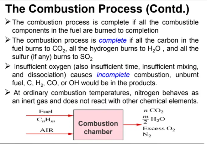
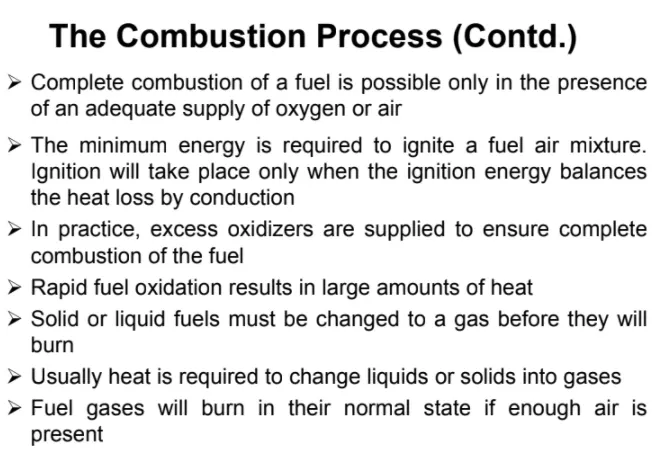
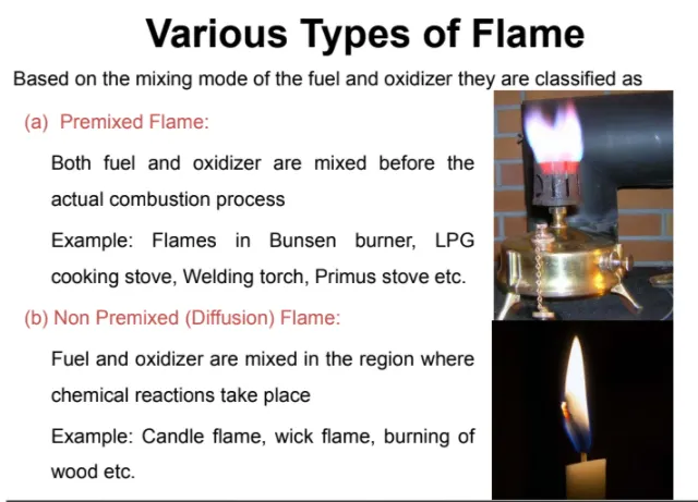
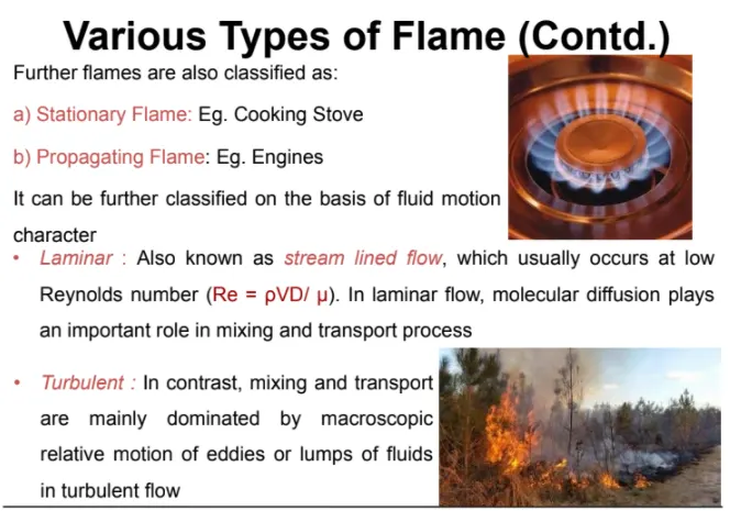
Combustion:
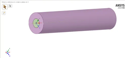
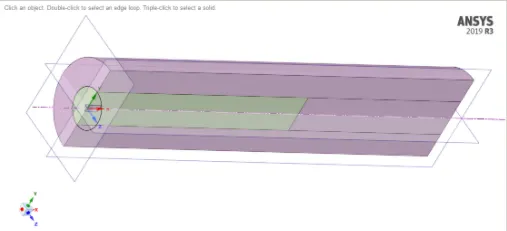
Geometry:
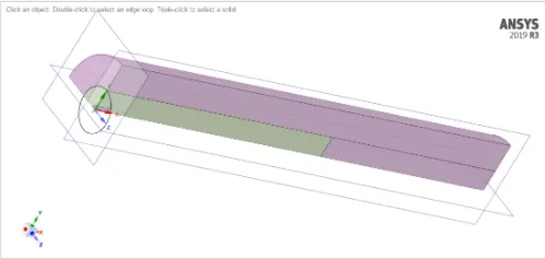
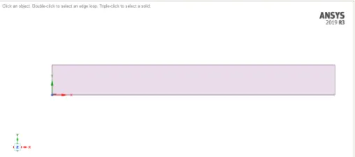
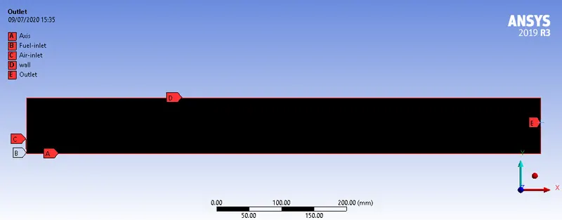
Only 1/4th part of model is used for analysis. Body split tool is used for splitting bodies. 2D front face is used for Analysis.
3D model:
2D Geometry:
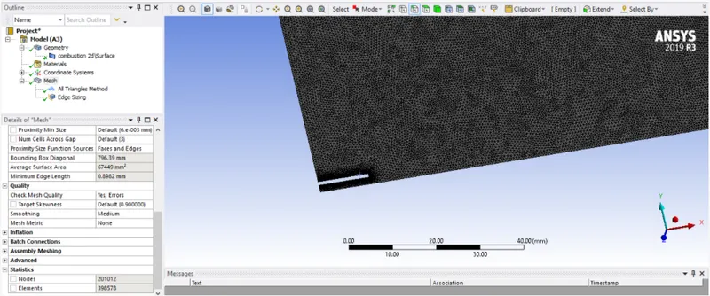
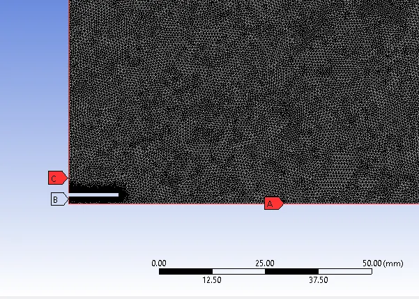
Meshing:
Element size of 1mm is use with capture proximity no. of cells at 5.
Case setup:
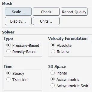
Solver: Pressure based, Steady state, Absolute and Axisymmetric
 t
t
Models:
Turbulence model: K-Epsilon model with standard wall functions
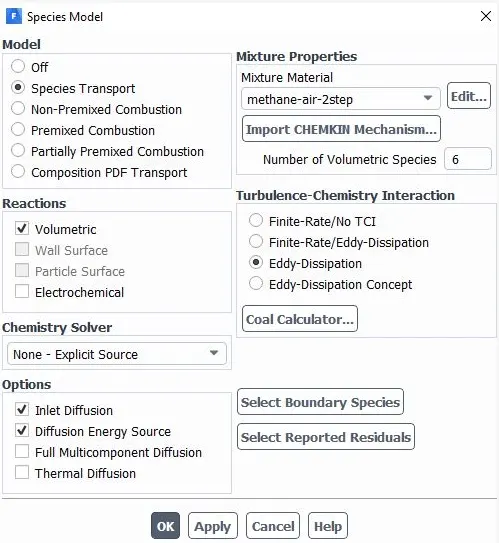
Species model turned ON:
Species model is enabled, and the species transport model is chosen.
Volumetric reactions are enabled.
Methane air 2 step is chosen as the mixture material.
Eddy-dissipation is chosen as the turbulence chemistry interaction.
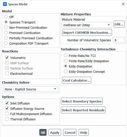
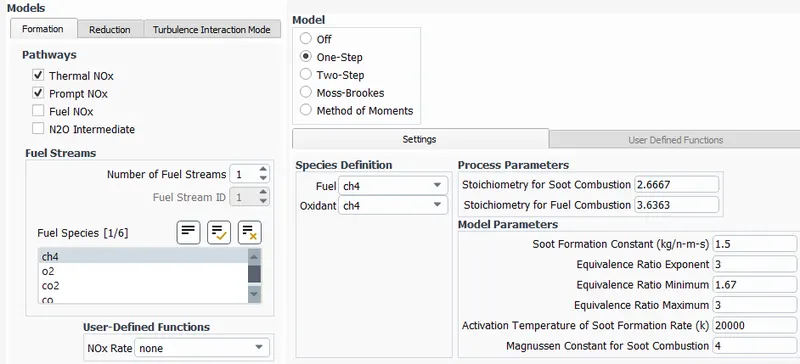
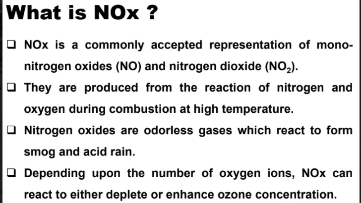
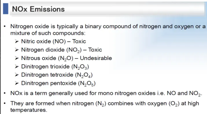
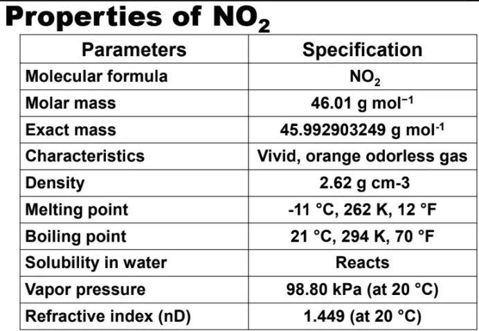
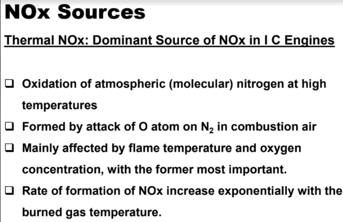
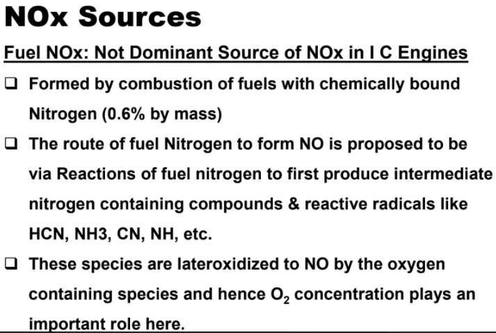
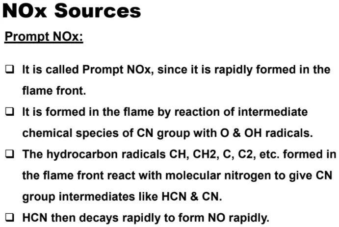
Model > Species > NOx Model > Thermal NOx > Promt NOx
Model > Species > Soot model > One step soot model
Boundary conditions:
Case 1:
As there is no addition of water, Air inlet will have velocity of 0.5 m/s with thermal temperature 300k with species of 0.23 mass fraction of O2.
For fuel inlet, velocity is 8 m/s with thermal temperature 300K and Species of 1 mass fraction of CH4.
Case 2:
There is addition of water in terms of 5 to 30 % in fuel. So all the above conditions remains same with only change in fuel inlet species of H2O with respect to CH4 mass fractions. Air inlet species remains same with 0.23 mass fraction of O2.
Solving Methods:
Hybrid Initialisation.
Running for 1000 iterations.
Case 1: CH4=1, O2 = 0.23
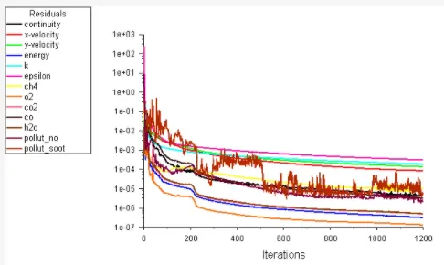
Residual Plot:
Contours:
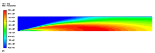
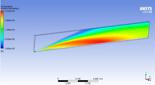
Static temperature:
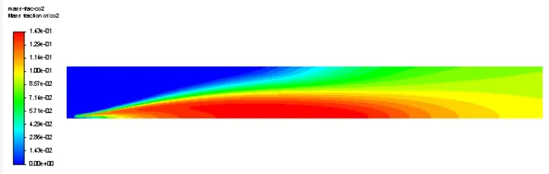
Mass fraction of CO2:
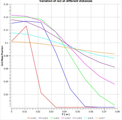
Variation of CO2 at different distances:
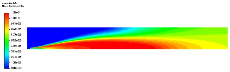
Mass fraction of H2O:
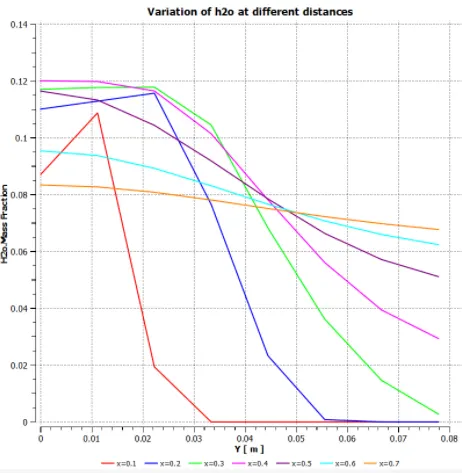
Variation of H2O at different distances:
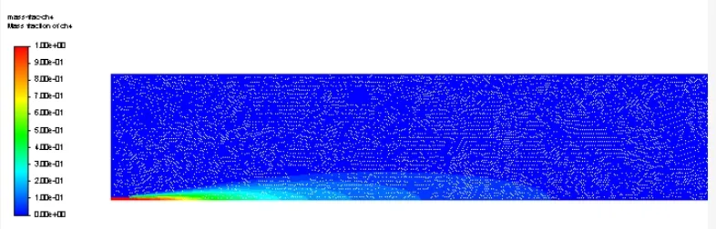
Mass fraction of CH4:
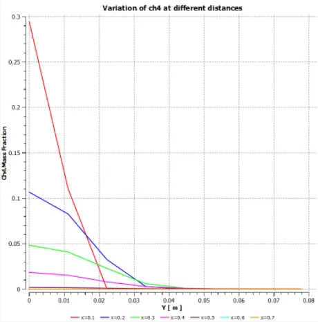
Variation of CH4 at different distances:
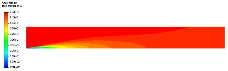
Mass fraction of N2:
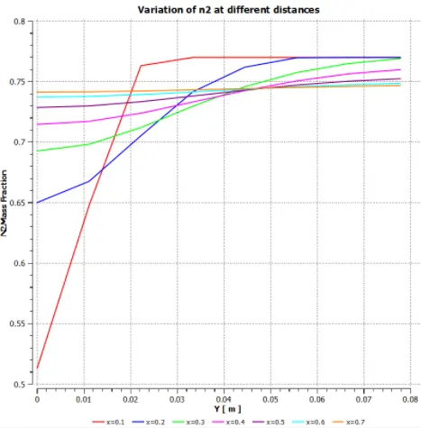
Variation of N2 at different distances:
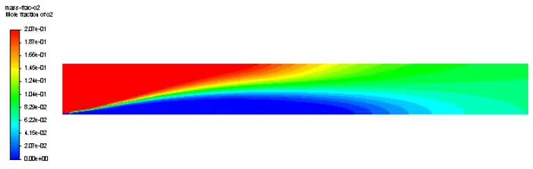
Mass fraction of O2:
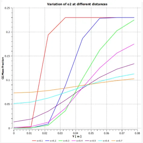
Variation of O2 at different distances:
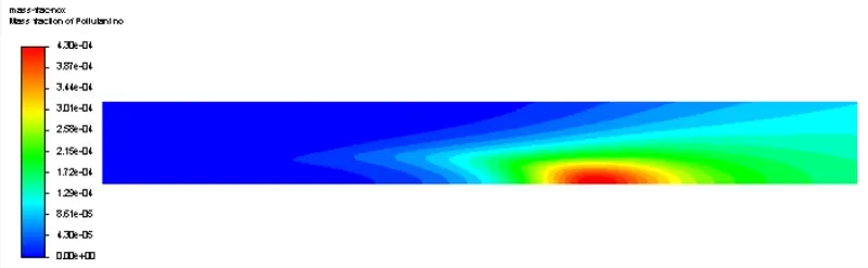
Mass fraction of NOx:
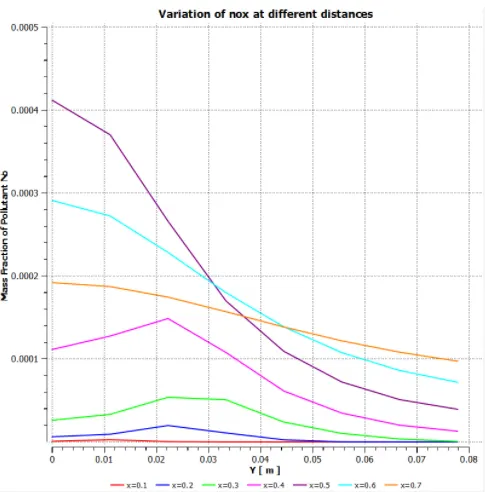
Variation of NOx at different distances:
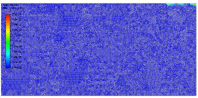
Mass fraction of Soot:
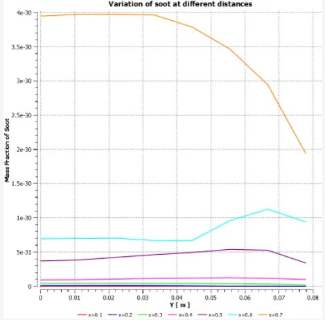
Variation of Soot at different distances:
Case 2:
a. CH4 = 0.95, H2O = 0.05
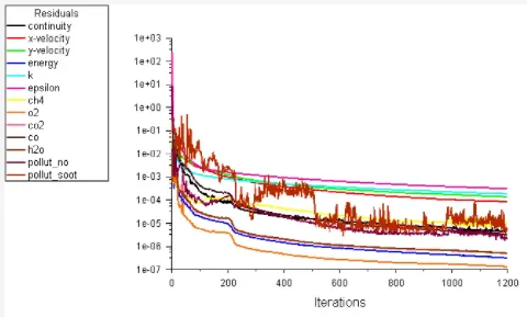
Residual Plot:
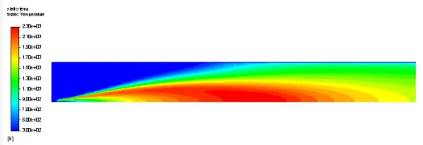
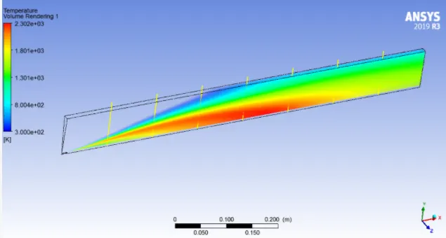
Static temperature:
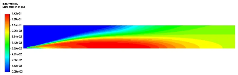
Mass fraction of CO2:
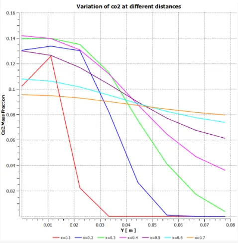
Variation of CO2 at different distances:
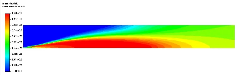
Mass fraction of H2O:
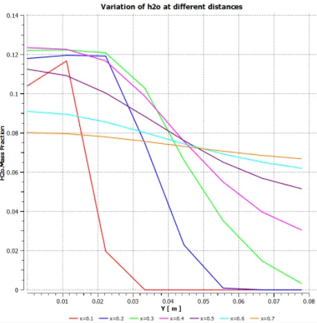
Variation of H2O at different distances:
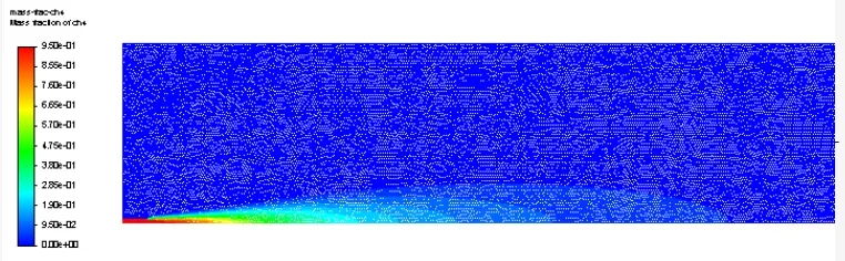
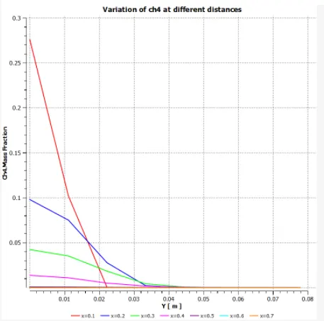
Mass Fraction of CH4:
Variation of CH4 at different distances:
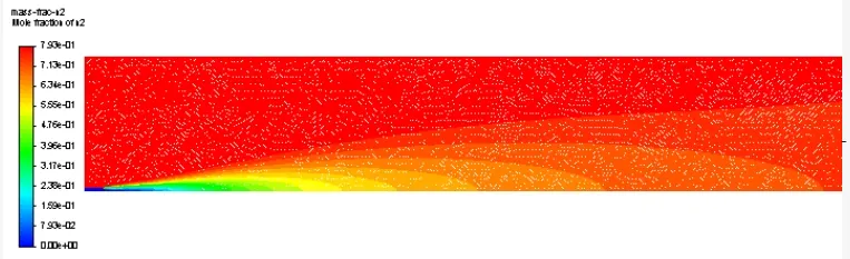
Mass fraction of N2:
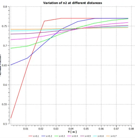
Variation of N2 at different distances:
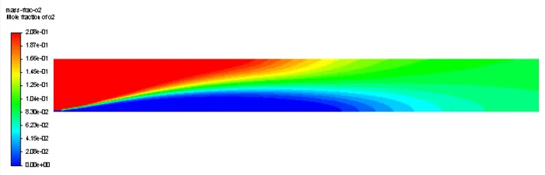
Mass fraction of O2:
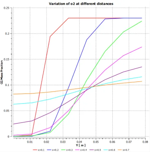
Variation of O2 at different distances:
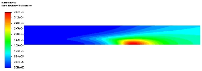
Mass fraction of NOx:
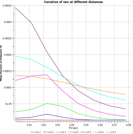
Variation of NOx at different distances:
Mass fraction of Soot:
Variation of Soot at different distances:
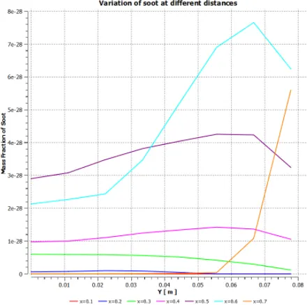
b. CH4 = 0.85, H2O = 0.15
Residual Plot:
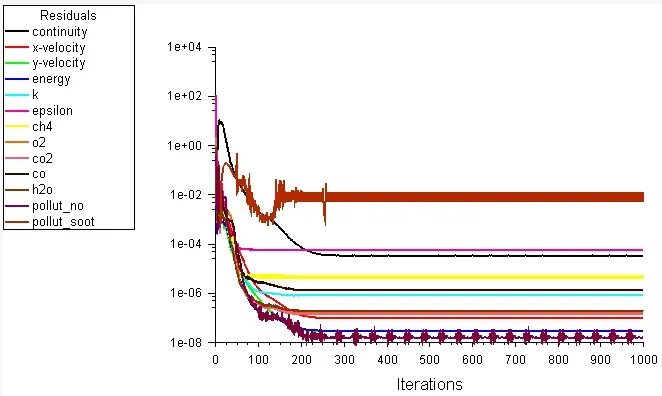
Static temperature:
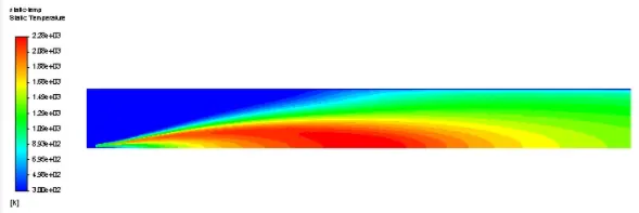
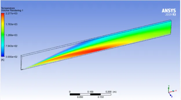
Mass fraction of CO2:
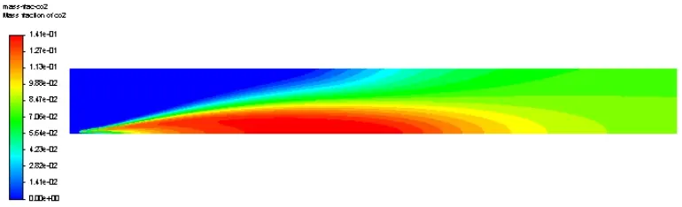
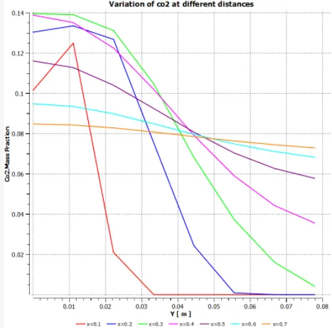
Variation of CO2 at different distances:
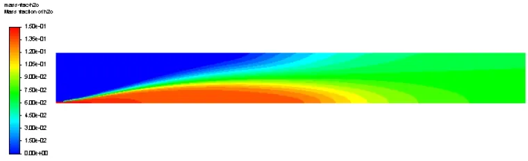
Mass fraction of H2O:
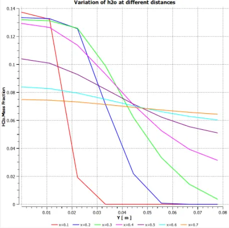
Variation of H2O at different distances:
Mass fraction of CH4: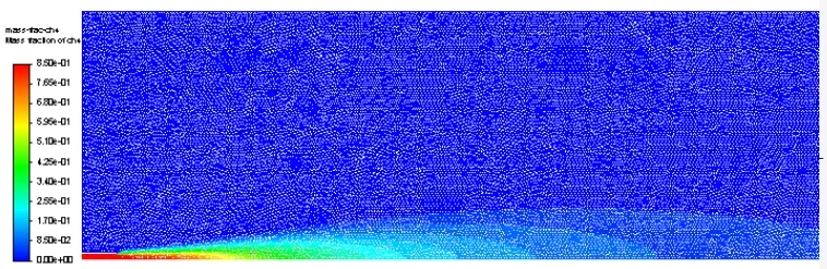
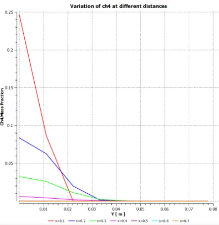
Variation of CH4 at different distances:
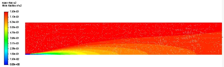
Mass fraction of N2:
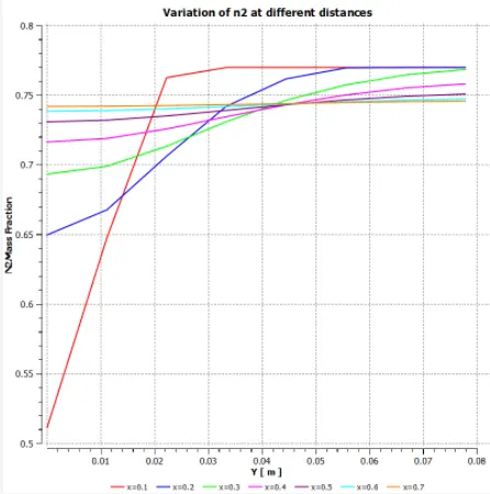
Variation of N2 at different distances:
Mass fraction of O2:
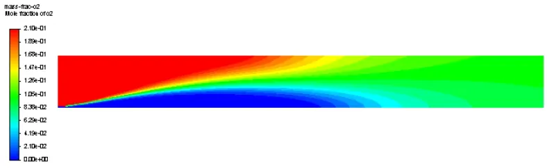
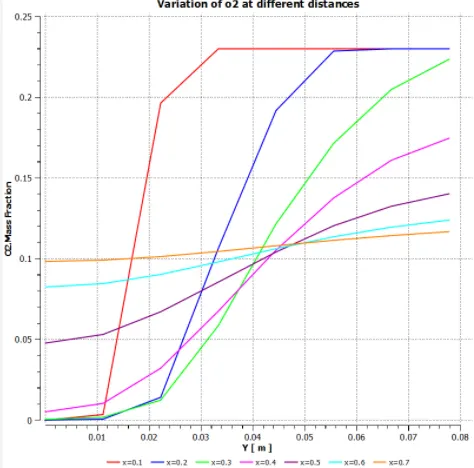
Variation of O2 at different distances:
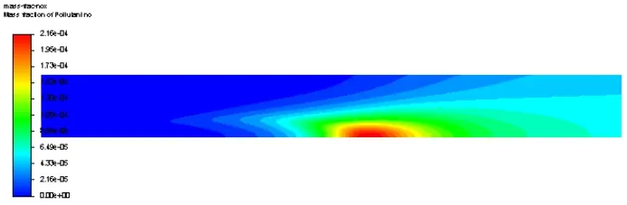
Mass fraction of NOx:
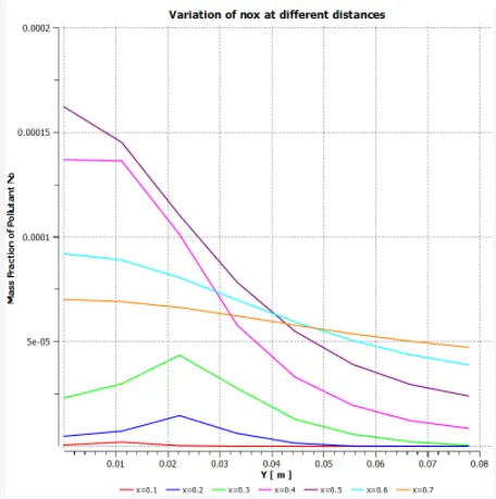
Variation of NOx at different distances:
Mass fraction of Soot:
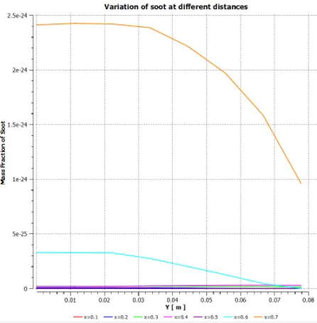
Variation of Soot at different distances:
c. CH4 = 0.75, H2O = 0.25
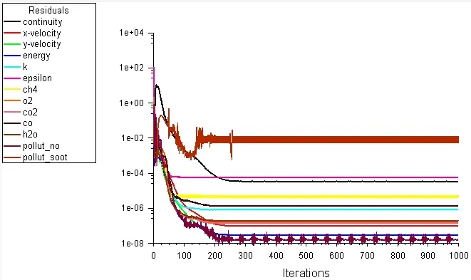
Residual Plot:
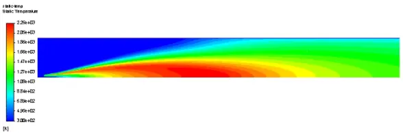
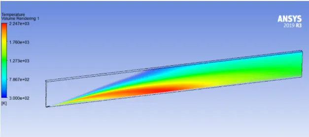
Static temperature:
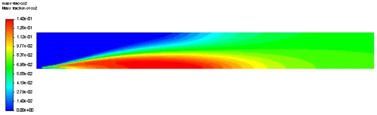
Mass fraction of CO2:
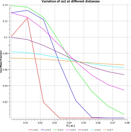
Variation of CO2 at different distances:
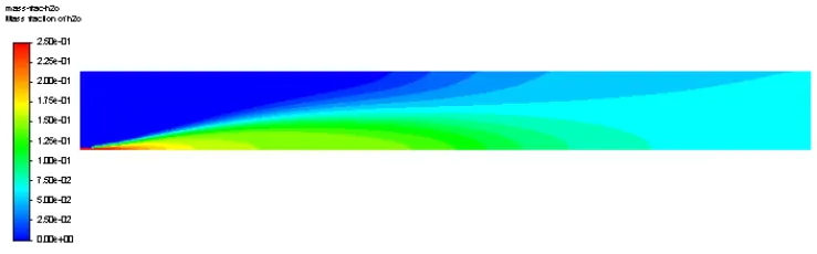
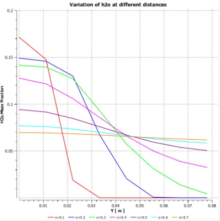
Mass fraction of H2O:
Variation of H2O at different distances:
Mass fraction of CH4: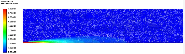
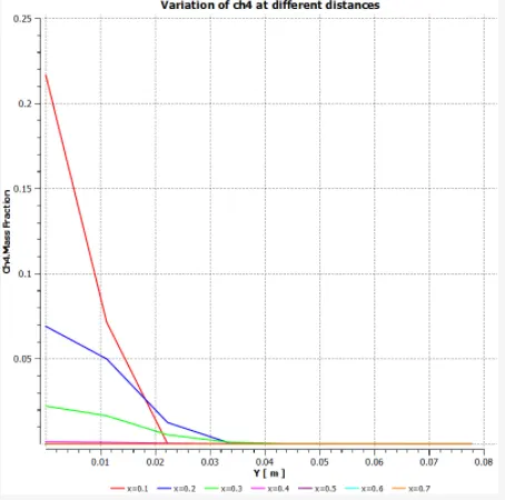
Variation of CH4 at different distances:
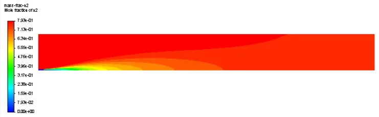
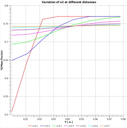
Mass fraction of N2:
Variation of N2 at different distances:
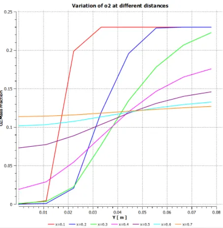
Mass fraction of O2:
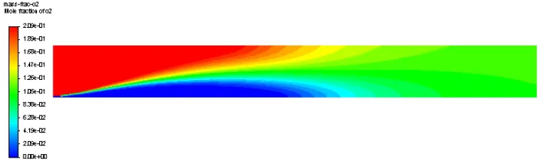
Variation of O2 at different distances:
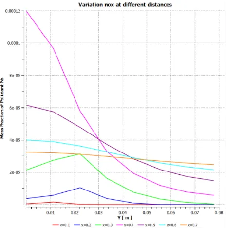
Mass fraction of NOx:
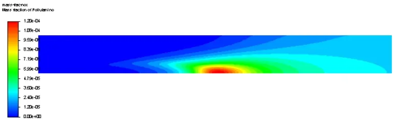
Variation of NOx at different distances:
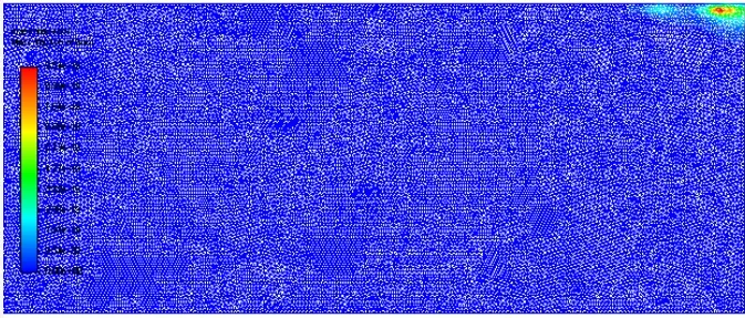
Mass fraction of Soot:
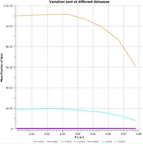
Variation of Soot at different distances:
d. CH4 = 0.7, H2O = 0.3
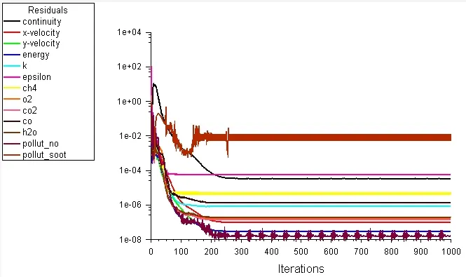
Residual plot:
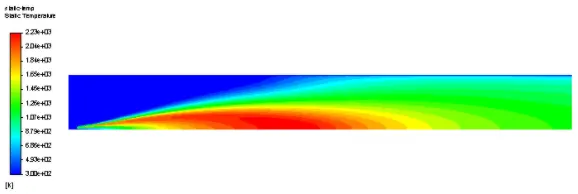
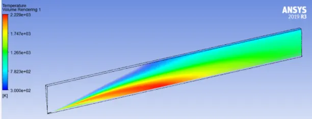
Static temperature:
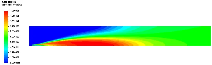
Mass fraction of CO2:
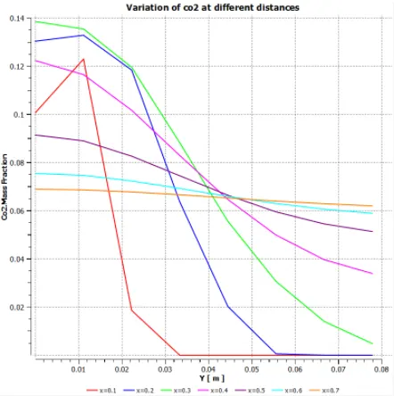
Variation of CO2 at different distances:
Mass fraction of H2O:
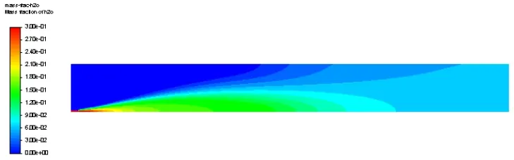
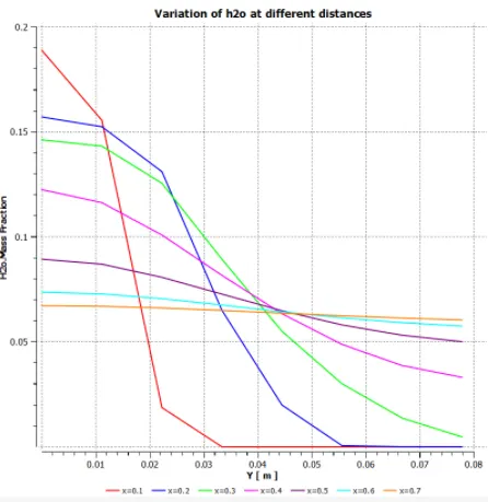
Variation of H2O at different distances:
Mass fraction of CH4: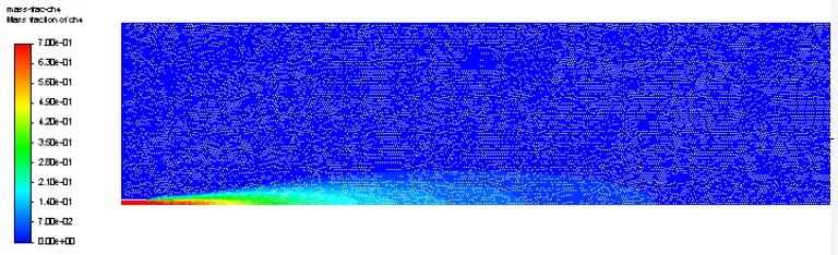
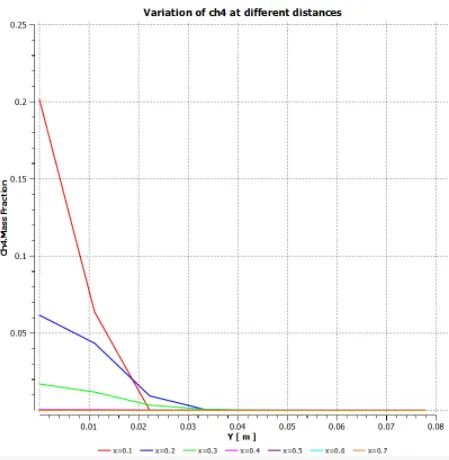
Variation of CH4 at different distances:
Mass fraction of N2:
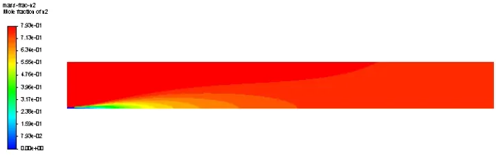
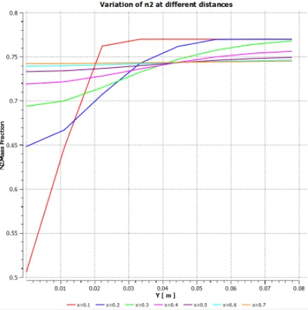
Variation of N2 at different distances:
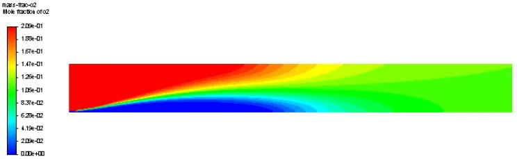
Mass fraction of O2:
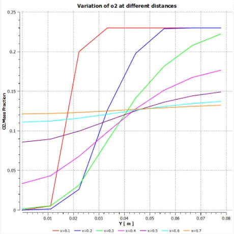
Variation of O2 at different distances:
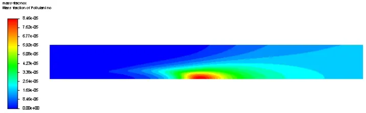
Mass fraction of NOx:
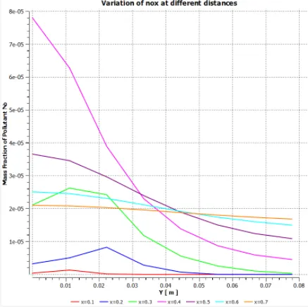
Variation of NOx at different distances:
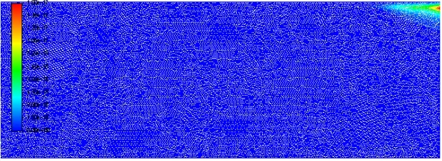
Mass fraction of Soot:
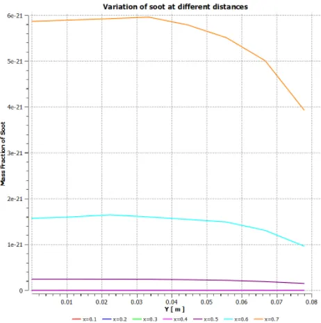
Variation of Soot at different distances:
Comparison of NOx and Soot mass fractions:
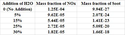
Graph between Mass fraction of NOx vs Addition of Water H2O:
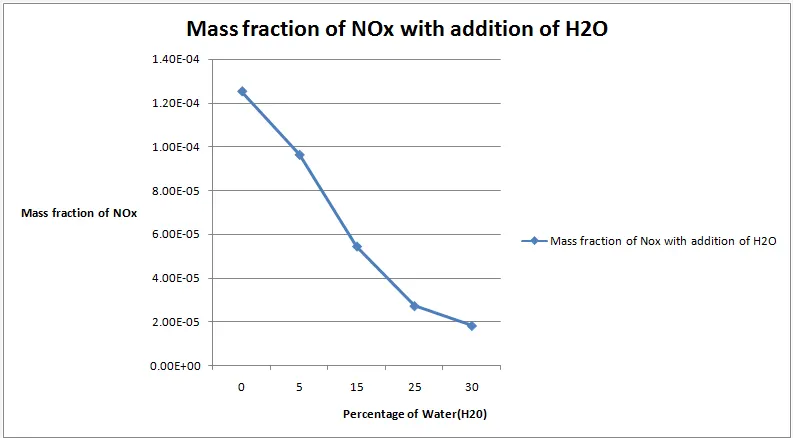
Graph between Mass fraction of Soot vs Addition of Water H2O:
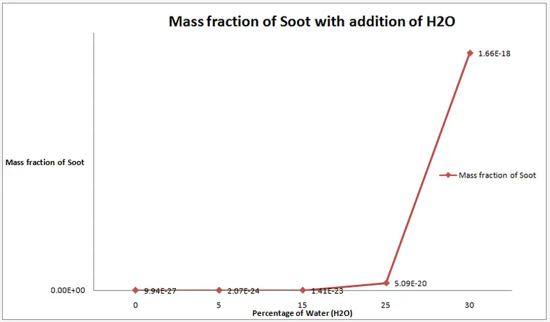
Conclusion:
From the above table and graphical representations, we can seen that the value of mass fraction of NOx decreases with increase in addition of water(H2O), Which is according to government norms with reduction of NOx formation.
We also observe that mass fraction of soot increases with increase in addition of water.
After running the simulation from both the parts, there are few conclusions that can be drawn out. the parts consist of different setup with the first being without the addition of H2O in fuel and second being with the different proportion of water in fuel from 5% to 30%.
The whole combustion simulation is done by the Eddy Dissipation model with the volumetric turned on. The model is used along with turbulence model.
The contour of Temperature, CO2 and H2O are more or less same which signifies than the species mass fraction depends on the effective combustion taking place. The formation of NOx is reduced as we increase the water content from 5% to 20% but in case of 30% the formation of NOx is more and also the soot which happens to be larger mass fraction than the previous cases.
With the addition of water the maximum temperature drops. The mass fraction of CO2 decreases whereas CO increases with the addition of water in the fuel.
NOx concentrations generated in the combustion are generally low. So it has little influence on the flow field and predictions, temperature and other combustion products.
Thus we can conclude that combustion simulation is performed successfully
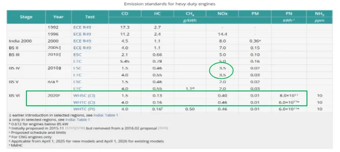
Referene Research Paper:
1. https://www.sciencedirect.com/science/article/pii/S1876610217337724
2. https://link.springer.com/article/10.1007/s00773-015-0303-8
3. Theory is taken from ARAI internal presentations.