Channel flow simulation using Converge CFD for different grid sizes
Aim: Study the Channel flow simulation using Converge CFD for diffrent mesh sizes
Software Used: Converge Studio
Objective:
1. Run the simulation for diffrent sizes
2. Contour plots of diffrent parameters
3. post process the results in Paraview and Converge post
Theory:
The analysis of flow patterns of water surface shape, velocity, shear stress and discharge through a stream reach falls under the heading Open Channel Flow.
Open Channel Flow is defined as fluid flow with a free surface open to the atmosphere. Examples include streams, rivers and culverts not flowing full. Open channel flow assumes that the pressure at the surface is constant and the hydraulic grade line is at the surface of the fluid
Steady and unsteady flow depend on whether flow depth and velocity change with time at a point. In general if the quantity of water entering and leaving the reach does not change, then the flow is considered steady.
Steady flow in a channel can be either Uniform or Non-uniform (varied).When the average velocities in successive cross sections of a channel are the same, the flow is uniform. This occurs only when the cross section is constant. Non-uniform flow results from gradual or sudden changes in the cross sectional area.
Channel Flow dimensions:
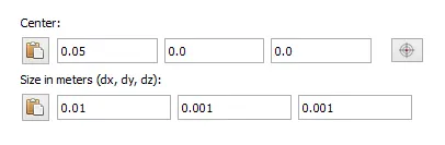
dimensions in meters
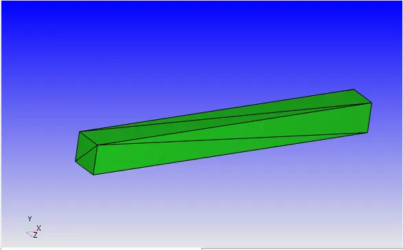
Geometry:
Case Setup:
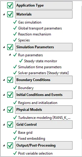
1. Application type: Time based-steady state
2.Materials : Air
Species : N2 and O2
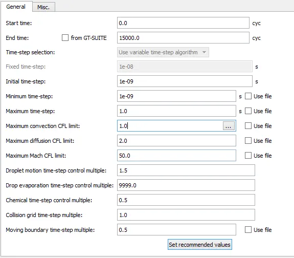
3.Simulation Parameters:
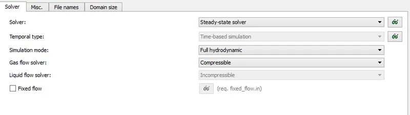
run parameters:
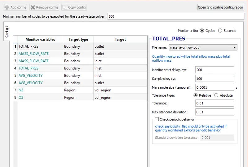
Steady State Monitor:
Simulation time parameters
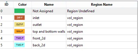
Boundary Conditions:
1.Inlet flow
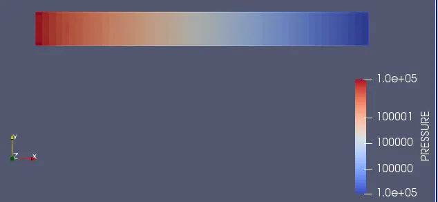
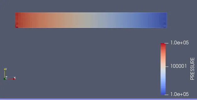
Pressure=100001 pa Temperature = 300k
2. Outlet flow
Pressure=100000 pa Temperature = 300k
3. Top and bottom walls = no slip condition
4. Front and Back 2D
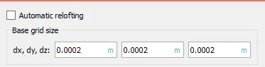
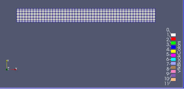
Mesh Sizes 1:
dx = 2e-4m, dy = 2e-4m, dz = 2e-4m
Velocity Vector:
Pressure Vector:
Plots:
Velocity:
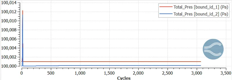
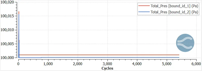
Pressure:
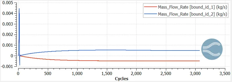
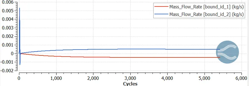
Mass Flow Rate:
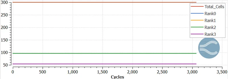
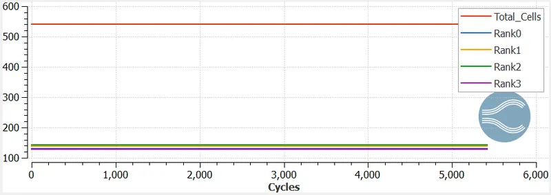
Total cell Count:
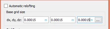
Mesh Sizes 2:
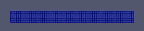
dx = 1.5e-4m, dy = 1.5e-4m, dz = 1.5e-4m
Meshing:
Contours:
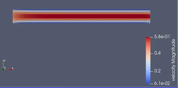
Velocity Contour:
Pressure contour:
Plots:
Velocity:
Pressure:
Mass flow rate:
Total cell count:
Mesh Sizes 3:
dx = 1.0e-4m, dy = 1.0e-4m, dz = 1.0e-4m
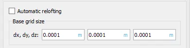
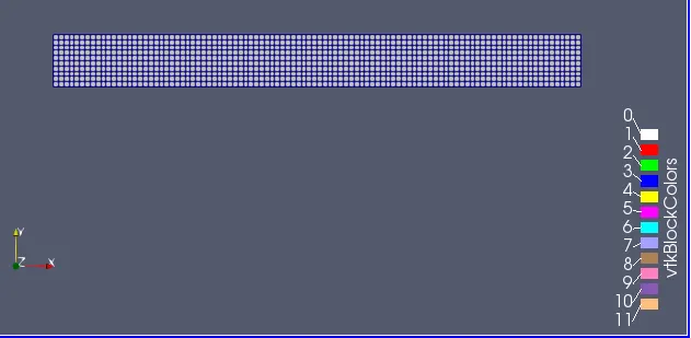
Meshing:
Contour:
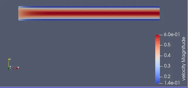
Velocity:
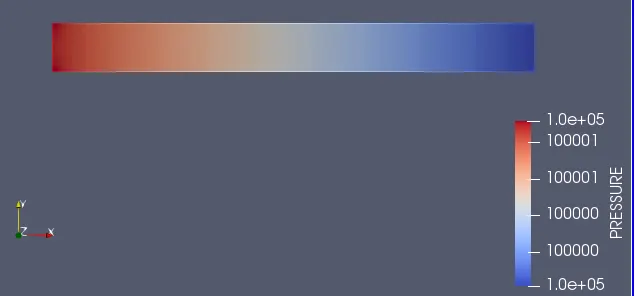
Pressure:
Plots:
Velocity:
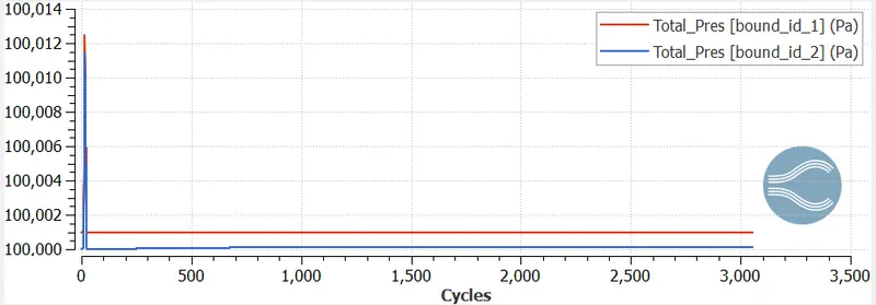
Pressure:
Mass flow rate:
Total Cell Count:
Conclusions:
The number ofcycles that each mesh case runs on the trasient on the problem and tolerance and sample size values are set in the solver.
For contour profiles we use the paraview post processer.
Comparing the plots and graphs for diffrent cases, accuracy of the solution increases when grid size is decreases.increase the no of cells computational time also increases exponentially.
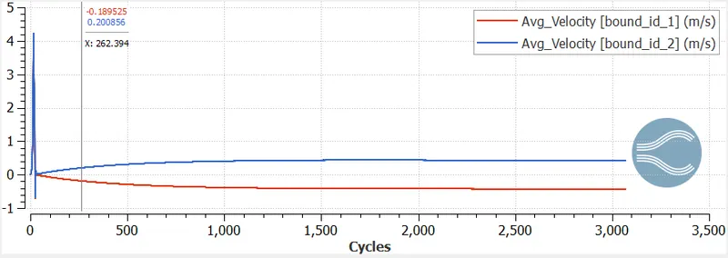
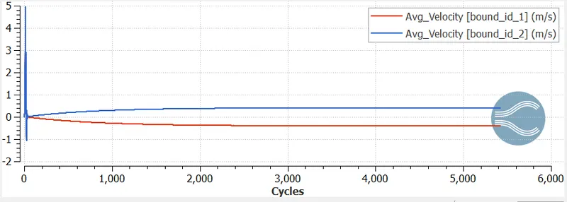
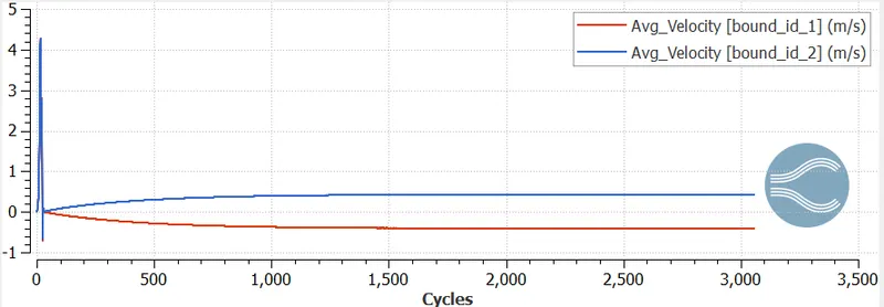
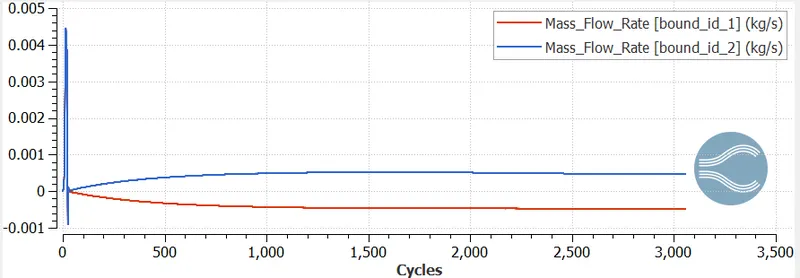
In the above plots their are two graphs for inlet and outlet,
in the inlet thier is a positive sign cause the flow along normal of the inlet boundary, outlet has converged to negative values as flow is opposite to direction.
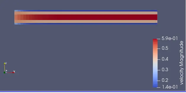
Velocity: During this simulation we observe that intially velocity should be high,After some cycles the solution get converge and it become stable.
velocity is zero at near the walls and maimum at centre axis of the channel.
maximum velocity is changes with respect to the change in mesh size.
Mass flow rate: mass flow at inlet and otlet is not same in the simulation
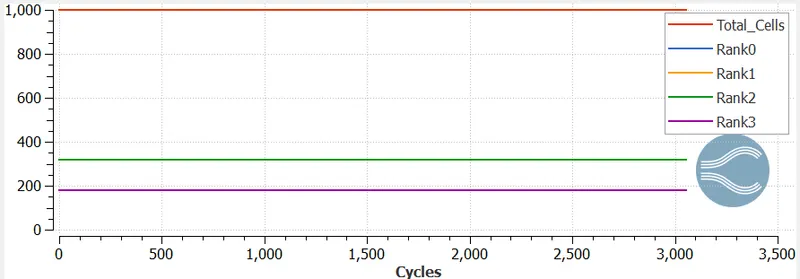
Total cell count:if we refine the grid size in difftrent cases, the total no of cells also increases .