Stalagmite function optimization using GA Algorithm.

Aim: write a code in MATLA to optimize the stalagmite function and find the global maxima of the function

Theory:

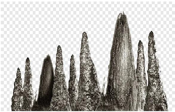
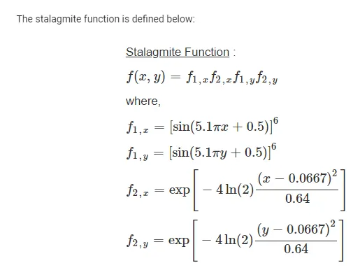
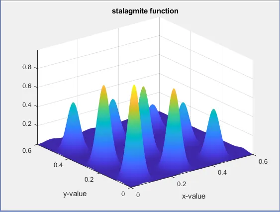
Stalagmite Function: stalagmite structures are formed from the caves floor that point upward.stalagmite functions are mathematical functions which represents shapessililar to that of stalagmite functions.

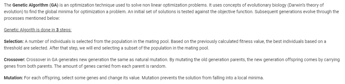
Genetic Algorithm:

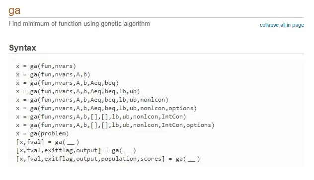
Syntax:

Software Used: MATLAB Programming

Program:

Code for stalagmite Function:

function[f] = stalagmite(input_vector)

x = input_vector(1);
y = input_vector(2);

f1 = (sin(5.1*pi*x +0.5)).^6;
f2 = (sin(5.1*pi*y +0.5)).^6;

f3 = exp(-4*log(2)*((x-0.0667).^2)/0.64);
f4 = exp(-4*log(2)*((y-0.0667).^2)/0.64);

f = -(f1*f2*f3*f4)
end

Main Program:

Stalagmite Function:

clear all
close all
clc

% defining your search space
x = linspace(0,0.6,150);
y = linspace(0,0.6,150);

% creating a 2D Dimensional mesh
[xx yy] = meshgrid(x,y);

tic

% evaluting Stalagmite function
for i = 1:length(xx)
for j = 1: length (yy)
input_vector(1) = xx(i,j);
input_vector(2) = yy(i,j);
f(i,j) = stalagmite(input_vector);
end
end

Study_time = toc

surfc(xx,yy,-f)
xlabel('x-value')
ylabel('y-value')
title('stalagmite function')

shading interp

Output Command:

Study_time =

5.8786

plot:

Study 1:

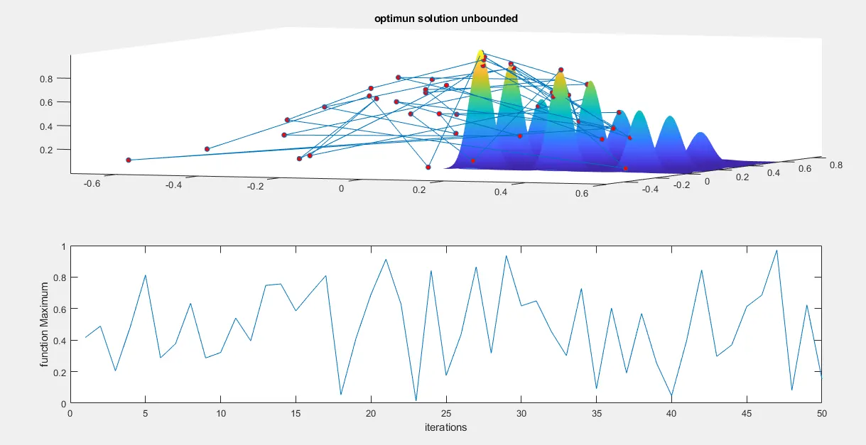
program for Unbounded:

% Unbouded Bhehaviour

tic

for i = 1: num_cases
[inputs,fopt(i)] = ga(@stalagmite,2);
xopt(i) = inputs(1);
yopt(i) = inputs(2);

end

study_time1 = toc

figure(1)
subplot(2,1,1)
hold on
surfc(xx,yy,-f)
shading interp
plot3(xopt,yopt,-fopt,'marker','o','markersize',5,'markerfacecolor','r')
title('optimun solution unbounded')
subplot(2,1,2)
plot(-fopt)
xlabel('iterations')
ylabel('function Maximum')

Output Command:

study_time1 =

53.7305

Plot:

Study 2:

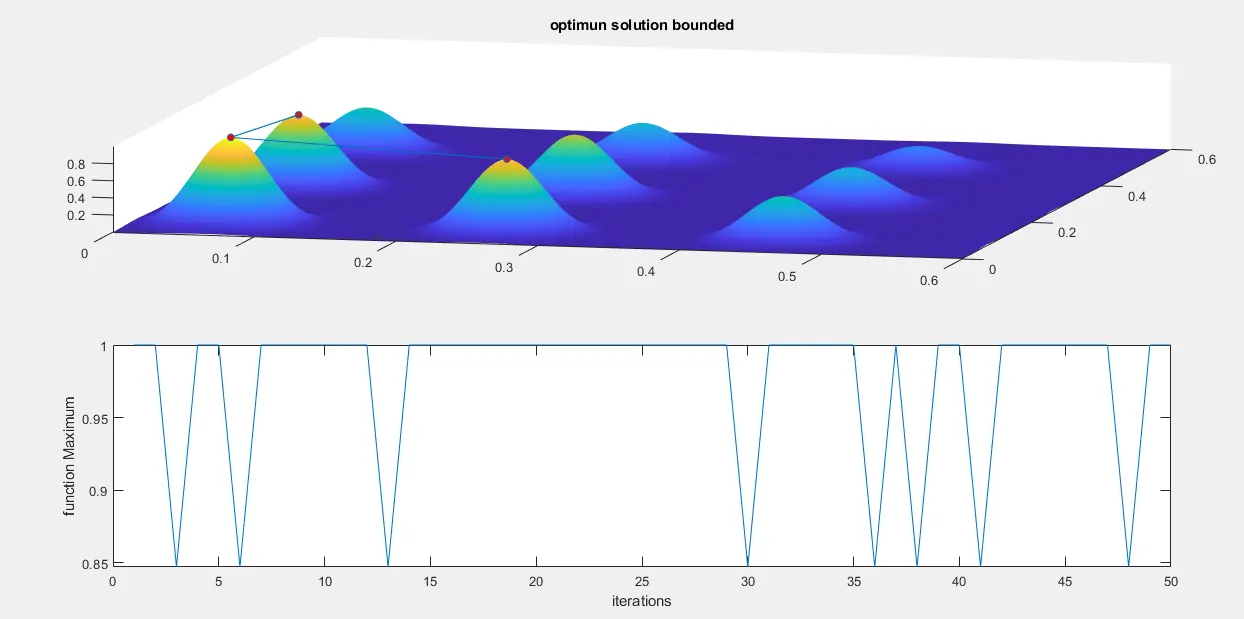
% Program for bounded(upper and lower bounded):

% bouded Bhehaviour

tic

for i = 1: num_cases
[inputs,fopt(i)] = ga(@stalagmite,2,[],[],[],[],[0,0],[0.6,0.6]);
xopt(i) = inputs(1);
yopt(i) = inputs(2);

end

study_time2 = toc

figure(2)
subplot(2,1,1)
hold on
surfc(xx,yy,-f)
shading interp
plot3(xopt,yopt,-fopt,'marker','o','markersize',5,'markerfacecolor','r')
title('optimun solution bounded')
subplot(2,1,2)
plot(-fopt)
xlabel('iterations')
ylabel('function Maximum')

Output Command:

study_time2 =

44.6541

Plot:

Study 3:

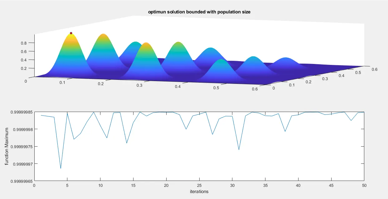
% bounded with population size:

% Bounded with population size

options = optimoptions(@ga)
options = optimoptions(options,'populationsize',170)

tic

for i = 1: num_cases
[inputs,fopt(i)] = ga(@stalagmite,2,[],[],[],[],[0,0],[0.6,0.6],[],[],options);
xopt(i) = inputs(1);
yopt(i) = inputs(2);

end

study_time3 = toc

figure(3)
subplot(2,1,1)
hold on
surfc(xx,yy,-f)
shading interp
plot3(xopt,yopt,-fopt,'marker','o','markersize',5,'markerfacecolor','r')
title('optimun solution bounded with population size')
subplot(2,1,2)
plot(-fopt)
xlabel('iterations')
ylabel('function Maximum')

Output Command:

study_time3 =

132.1473

Plot:

Note:

what are information i write in theory under the reference of Skill lync and wikipedia.