Assignment 6-Frontal Crash Simulation Challenge

1. Objective:

To perform a frontal crash with the help of a given car model. To obtain the results as mentioned in the above question, the following steps should be followed:

• To change the center of gravity from initial position to the required position.
• To check for the penetrations.
• To create new interfaces.
• To create accelerometers at the base of B-pillar to obtain the acceleration.
• To assign the initial velocity.
• To create the springs to obtain intrusions.
• To create the type 7 contact at front to obtain the axial force recieved on the rails from bumper.
• To create a rigid wall.
• To create the TH for all inputs. Inorder to obtain outputs.
• To run the simulation.
• To plot the graphs with the obtained results(Post-processing).

2. Software used: Altair Hyperworks Desktop 2020

3. User profile: Radioss

4. Abstract:

Now-a-days the vehicles are increasing day-by-day. And the companies are designing the automobiles by collecting the data from customer requirements & features. In that scenario, Now-a-days a car with crash proof when compared to other cars in the market will have demand. Keeping that in mind, the companies are performing several crash tests such as frontal crash, side crash, roof crash. Among them, frontal crash occurs frequently. So, the automotive companies are investing a lot for performing several analysis.

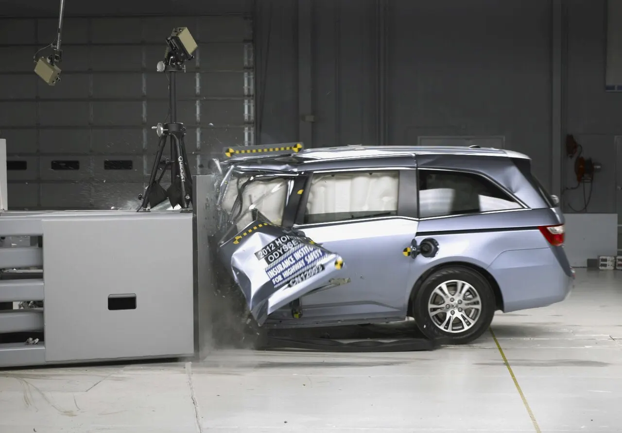
In that aspect, the frontal crash is performed in this project with the help of hypercrash as pre-processor & radioss as solver. The simulation is done here, Which would replicate the real world scenario. In this project, several things such as interfaces, accelerometers(For obtaining the acceleration), sections(for obtaining the forces passing though that sections), springs(To find the intrusions), rigid wall,assigning the initial velocity. And the simulation is runned. And the obtained outputs are plotted in the form of graphs. Which depicts the various parameters such as intrusions, forces in various components of the car. Which would replicate the real world scenario.

5. Procedure:

Step 1: Changing the initial position of center of gravity(COG) to the required position:-

Initially, The given model is opened in hypercrash. To change the COG. As the hpercrash is a pre-processor , the solver deck can be set up. To open hypercrash, the process is: Open Altair Hyperworks Desktop software---> Choose Applications option in menu bar(as shown in fig 5.1)---> Select the "Hypercrash" option in it.

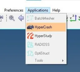
fig 5.1

After choosing the hypercrash option, a pop-up appears as shown in fig 5.2. In order to choose the unit system. The most widely used uinit systems is (KN, mm, ms, Kg).

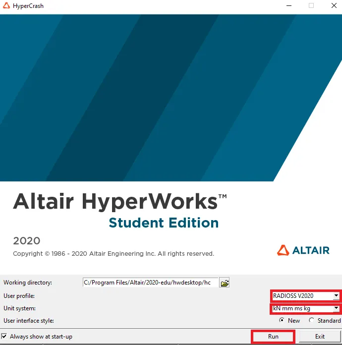
fig 5.2

After selecting the unit system, it takes some time to open. After opening, the hyperworks graphical interface appears as shown in fig 5.3.

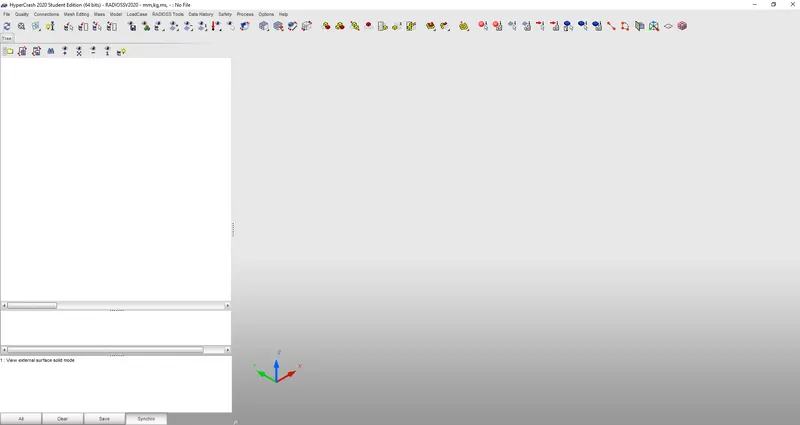
fig 5.3

Then the file is imported. After importing the model, it appears as shown in fig 5.4.

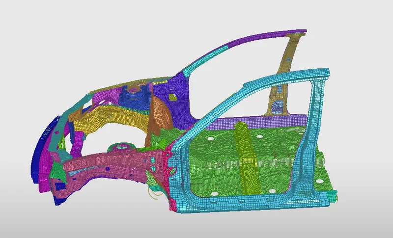
fig 5.4

Inorder to view the mass and center of gravity. an option named "mass" in the menu bar is choosed. In that, the "balancing" option is choosed as shown in fig 5.5.

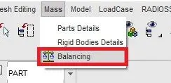
fig 5.5

After choosing that, an option which is highlighted in the fig 5.6 is choosed. Which depicts to view the COG.

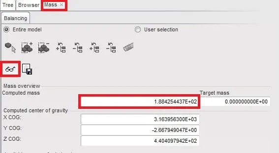
fig 5.6

After choosing this option, the initial position of COG appears as shown in fig 5.7.

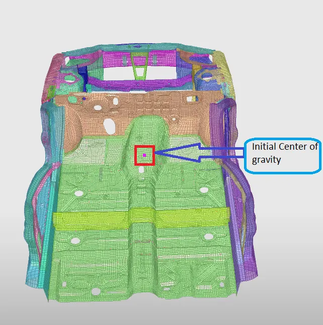
fig 5.7

Then the masses should be added. Inorder to bring the COG to the center of the cross member. For doing that, the process is: Loadcase option in menu bar(as shown in fig 5.8)---> select the option "Added mass".

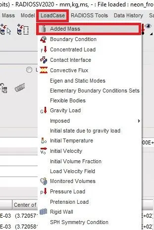
fig 5.8

Then to add the mass, by right clicking on the tab bar, a pop-up appears as shown in fig 5.9. Which indicates creating the mass by choosing the type 1.

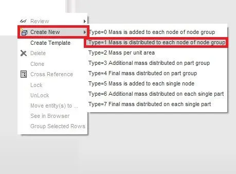
fig 5.9

Then the nodes are selcted to assign the mass from the graphical display, as shown in fig 5.10.

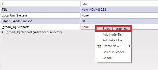
fig 5.10

After selecting the option from graphics, a pop-up appears as shown in fig 5.11. Which depicts to add or remove the nodes.

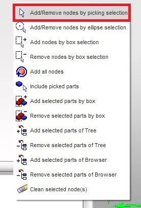
fig 5.11

After selecting that option, the selected nodes appears in red colour as shown in fig 5.12. After selecting the nodes, an option "Yes" at the right side bottom corner should be clicked, inorder to save them.

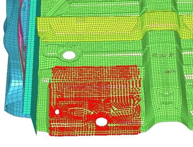
fig 5.12

After adding the mass to that nodes, the COG is viewed again. Now the postion of COG is changed when compared to the previous. The obtained COG position appears as shown in fig 5.13.

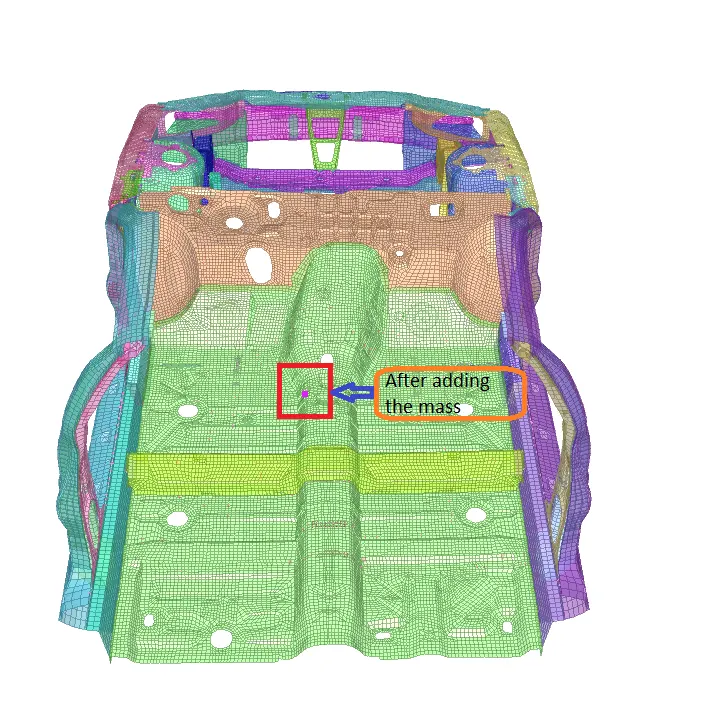
fig 5.13

SImilarly, the nodes are selected on the other side of the model, as shown in fig 5.14. Inorder to change the postion of COG to the required position.

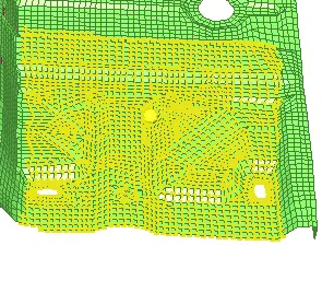
fig 5.14

Then again the COG is viewed. The change in COG position appears as shown in fig 5.15.

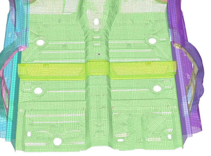
fig 5.15

Some more mass is added at the front side also. After adding the masses then to know how much mass is added, The process is: Select "mass" option---> Then we can see the mass value as 700.4 Kg. As shown in fig 5.16.

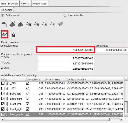
fig 5.16

After attaining the 700 kg mass, Then again COG is viewed. Now the obtained COG position is the required postion(i.e., At the middle of cross member). As shown in fig 5.17.

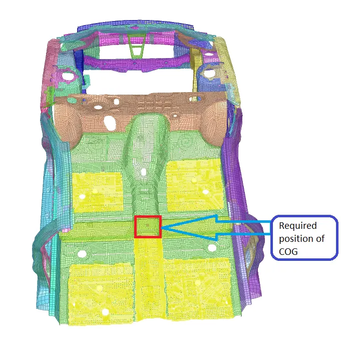
fig 5.17

The next step is to save this file and export to any location. Then the exported file is imported in to hypermesh, to run the simulation. As shown in fig 5.18.

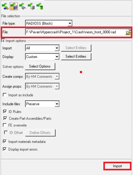
fig 5.18

After importing the model in to hypermesh, the model in the graphical display appears as shown in fig 5.19.

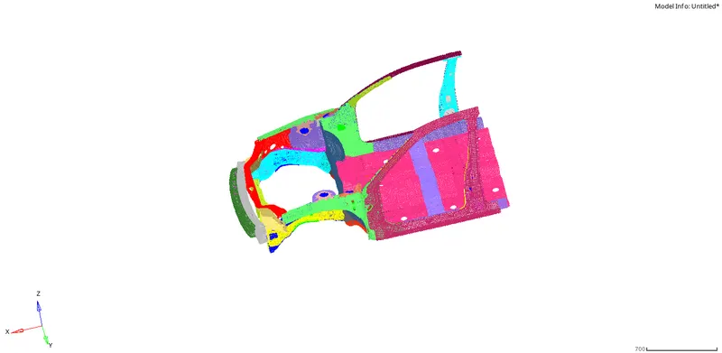
fig 5.19

To get a clarity regarding the mass of the imported model, Whether the model possesses the sam mass or not? Then it is checked by selecting the option "Tools" from menu bar---> In that select the option "Mass Details"---> "Mass,Cog & Inertia, as shown in fig 5.20.

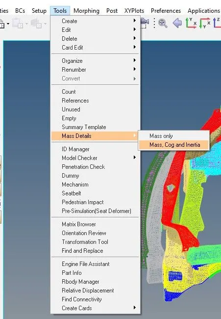
fig 5.20

After selecting that option, the total mass of the model can be viewed. As shown in fig 5.21. The seen mass is same as that of in the hypercrash. Which indicates, it's good to go.

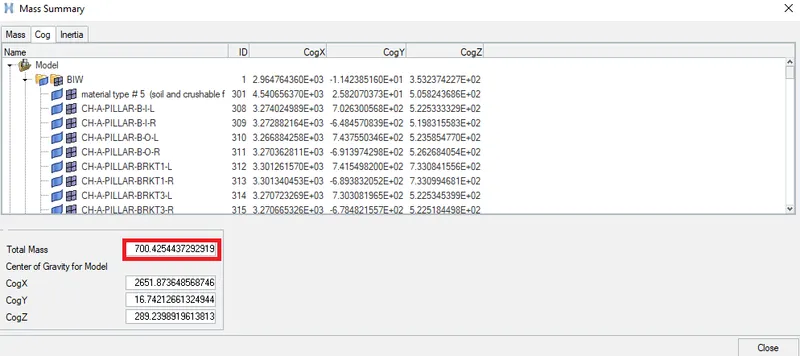
fig 5.21

Step 2: Check for penetrations:-

In this step for checking the penetrations, the process is: select "Tools" option in menu bar---> Select penetration check. As shown in fig 5.22.

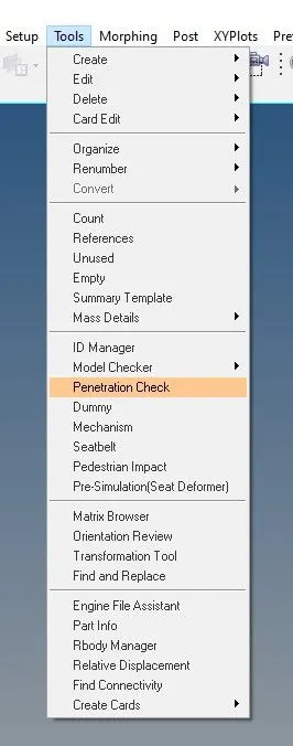
fig 5.22

After selecting that, the interfaces(Groups) should be defined, as shown in fig 5.23. Then by clicking on "Check", the solver checks for any pentrations. If there are any penetrations, it will show. Or else, it will show no penetrations as shown in fig fig 5.23.

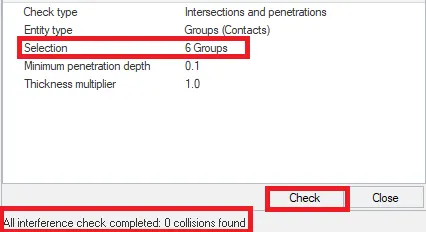
fig 5.23

Step 3: Creating the interfaces:-

In this step, the interfaces are created. Initially, the type 7 contact is created with the recommended values, as shown in fig 5.24.

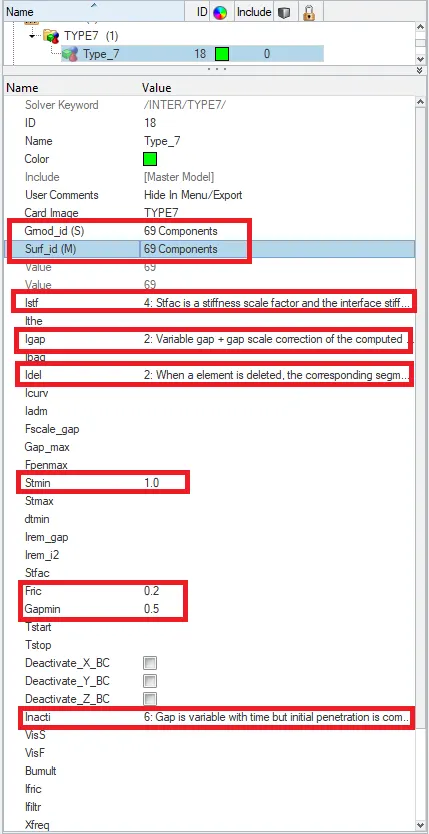
fig 5.24

Step 4: Creating the sections:-

In this step, the sections are created. As mentioned in the question, a section should be created at the node 174247. So, for finding that node an option "Display numbers" which is at the left side of the graphical display is choosed. As shown in fig 5.25

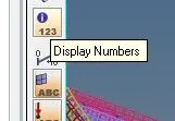
fig 5.25

After selecting that, the display numbers panel appears as shown in fig 5.26. For displaying that node, the process is: Nodes in display numbers panel---> Select node by Id(by right clicking in nodes)---> Click the option "ON". To view the node.

fig 5.26

The node required is shown, which is highlighted as shown in fig 5.27

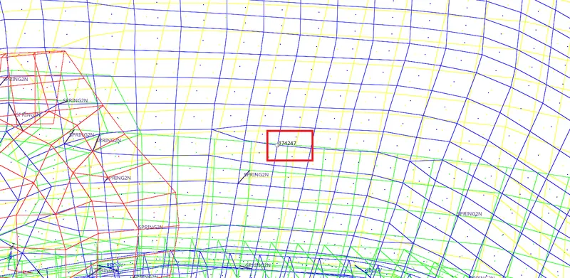
fig 5.27

For creating a section, a frame is needed. Which is a movable frame. So to create a frame, the process is: Right click on the tab bar in solver browser---> Create---> Frame---> Mov. As shown in fig 5.28.

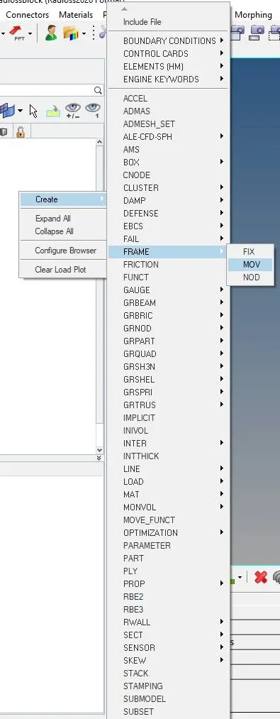
fig 5.28

After selecting that, at the bottom there will be a panel as shown in fig 5.29. Indicating to select the nodes, the 174247 node is selected as a origin. Then the next node specifies the Z-axis. And the third node depicts the YZ-plane. By clicking "create", a frame is created.

fig 5.29

The created frame at that node, appears as shown in fig 5.30.

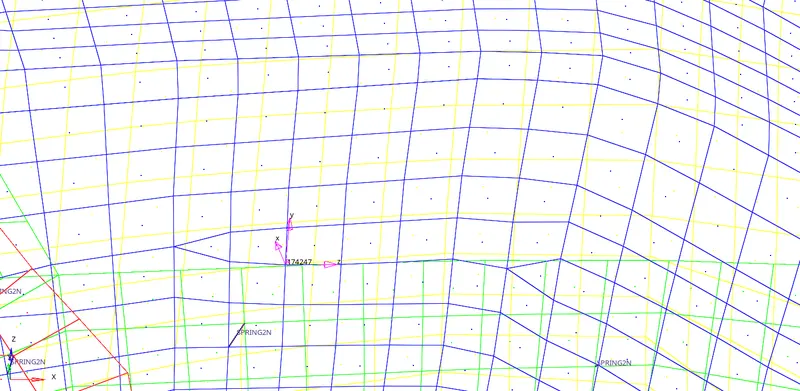
fig 5.30

Then a section is created. The process of creating the section is: Right click on the tab bar in solver browser---> Create---> SECT. As shown in fig 5.31.

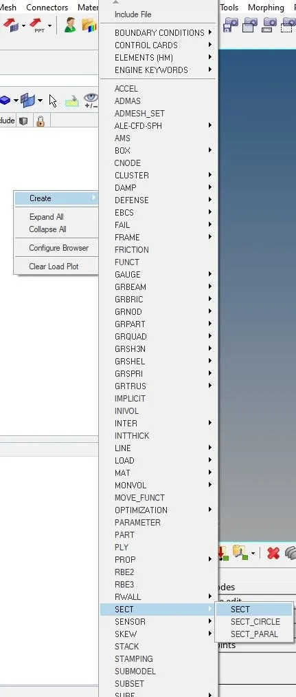
fig 5.31

After selecting that, the parameter table appears at the left bottom corner. In which the parameters such as nodes(N1,N2,N3), specifying the frame, Coeffifient for filtering(alpha= 0.67), Time step for saving the data(Delta T= 0.01), elements near to the frame(To view the section in terms of elements). As shown in fig 5.32.

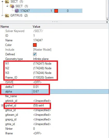
fig 5.32

The created section appears as shown in fig 5.33. This can be seen by right clicking on the created section And selct the option "isolate only".

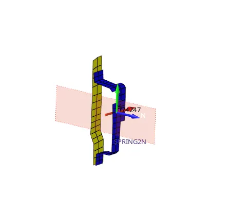
fig 5.33

In the same way a temp node is created at the 174247 node. And it is duplicated. Then it is translated to the opposite side. In order to create a section approximately in the other side of the rail. After translation it, the node appears near to the bolt connection, as shown in fig 5.34. So, a sectiom is created near to that node. This is done to compare the results at the end.

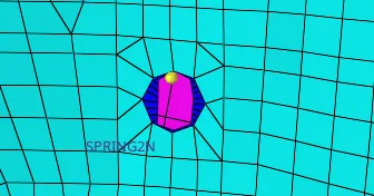
fig 5.34

Then a frame is created at any node. But it should be approximately near to the translated node. The created frame in that region appears as shown in fig 5.35.

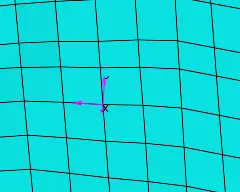
fig 5.35

Then a section is created. After craeting a section, it appears as shown in fig 5.36.

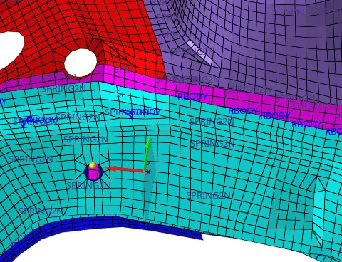
fig 5.36

Similarly, the sections should be created at the A-pillar & short gun for both sides. After creating all sections, the given model appears as shown in fig 5.37.

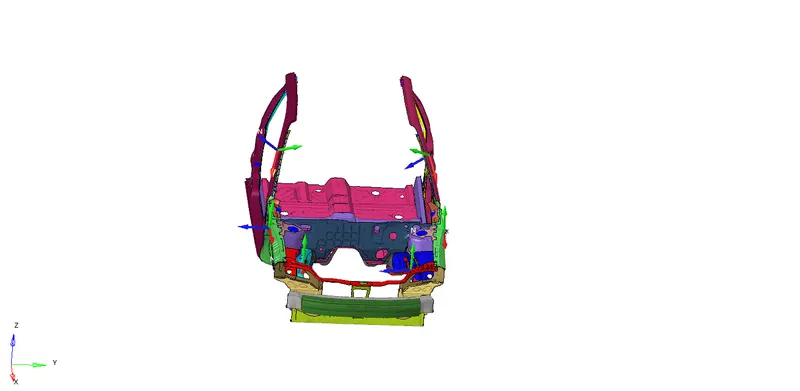
fig 5.37

Step 5: Creating accelerometer at B-pillar:-

In this case, the accelerometers are created at the B-pillar for both sides. In this challenge, the accelerometers are created at the rockers. Because, it will also show the same results. The process of creating the accelerometer is: Right click on the tab bar in solver browser---> Create--->Accel. As shown in fig 5.38

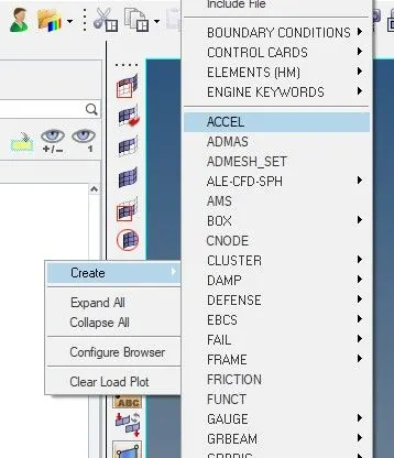
fig 5.38

Then the node should be selected(The node can be any, But at the middle of the rocker) in the parameter panel, as shown in fig 5.39.

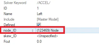
fig 5.39

After creating the accelerometer, it appears as shown in fig 5.40.

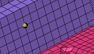
fig 5.40

Similarly, the accelerometer is created on the other end. Just as similar to translating the node, in the case of sections.

Step 6: Giving the initial velocity:-

In this case, the initial velocity is given to the model. In order to hit the model with the rigid wall. So to create it, the process is:Right click on the tab bar in solver browser---> Create---> Boundary conditions---> INIVEL. As shown in fig 5.41.

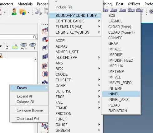
fig 5.41

Then in the parameter panel, the velocity components are entered, As shown in fig 5.42. In which the initial velocity assigned is 15.646 m/s(Which is equal to 35 mph).

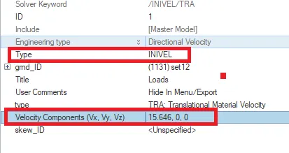
fig 5.42

After creating the initial velocity, it appears as shown in fig 5.43.

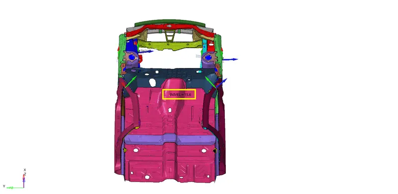
fig 5.43

Step 7: creating springs to obtain the intrusions:-

In this case, the springs are created at the mentioned nodes(66695,66244), to find the intrusions. The process of creating the springs is: 1D panel---> Springs---> Spring2(Springs with 2 nodes)---> Select two nodes---> Click on create. As shownin fig 5.44. In which one node is specified in the question. the other node is taken by the user. Same in the case of second spring also.

fig 5.44

After creating the springs at the specified nodes, it appears as shown in fig 5.45.

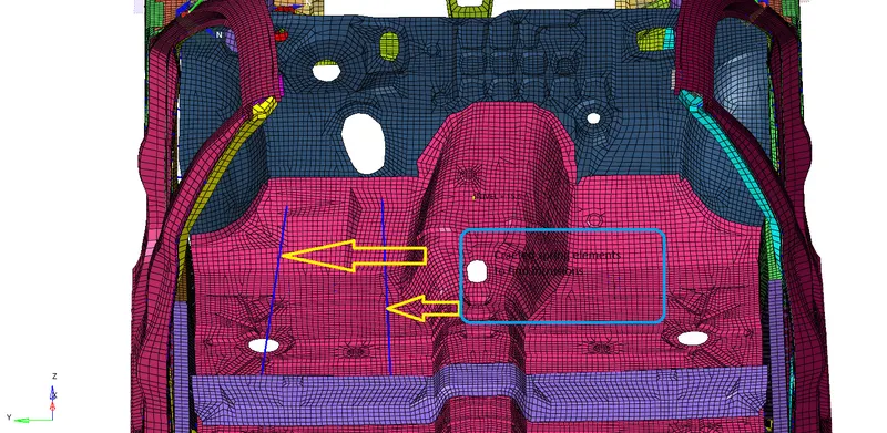
fig 5.45

Step 8: Create Type 7 contact at front:-

Iin this case, the interfaces are created at the front part of the model(i.e., near the bumper). Inorder to obtain the axial force received on the rails from bumper. So, the slaves nodes are selected first( Which is the component back of the bumper). As shown in fig 5.46.

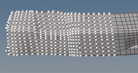
fig 5.46

After adding the slave nodes, the selected slave nodes appears with the reprsentation as shownin fig 5.47.

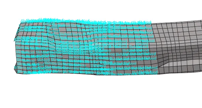
fig 5.47

Then the master elements are selected(Which acts as a master). After selecting some elements in the bumper as master, it appears as shown in fig 5.48.

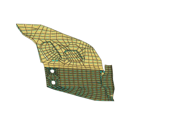
fig 5.48

Step 9: Creating a rigid wall:-

In this case, a rigid wall(with infinite plane) is created. And the process to create the rigid wall is: Right click on the tab bar in solver browser---> Create--->RWALL---> PLANE. As shown in fig 5.49.

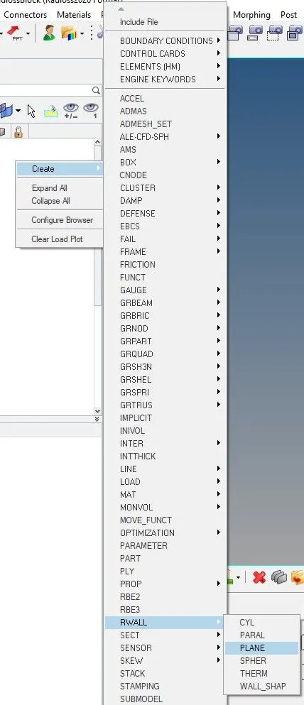
fig 5.49

Then two nodes are selected on the bumper to create the plane for defining the rigid wall, as shown in fig 5.50.

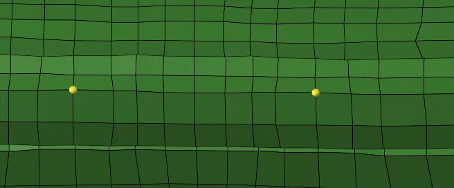
fig 5.50

Then translate one node, as shown in fig 5.51.

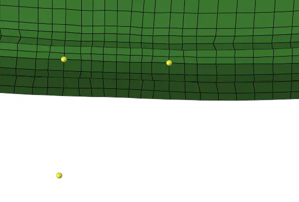
fig 5.51

Then duplicate the translated node twice. And Translate those duplicated nodes, One in y-axis & one in Z-axis. And translate the first node to half of the distance in y-direction, as shown in fig 5.52.

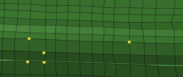
fig 5.52

Then in the parameter panel to specify the dimensions for creating the rigid wall, Some values should be specified. Such as (XM, YM, ZM) is specified by selecting the first translated node(Which acts as a origin), Normal is specified by selcting the three translated nodes as a plane. By switching the slide option to 2, the friction option will be enabled. And the friction value given is 0.1(as mentioned in the question). As shown in fig 5.53.

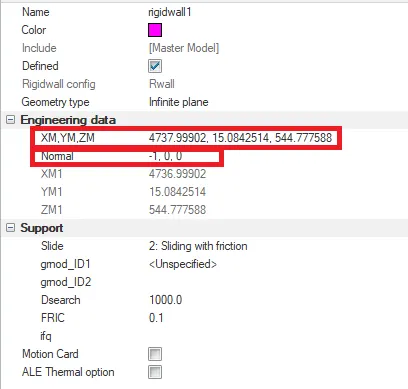
fig 5.53

After entering the values, the created rigid wall appears as shown in fig 5.54.

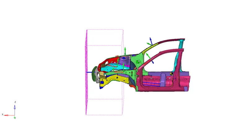
fig 5.54

Step 10: Giving the time step & creating TH:-

In this step, Initially the time step is assigned to the simulation. By entering the time step value as 0.0005 ms in the card named "DT/NODA", from the model browser, as shown in fig 5.55.

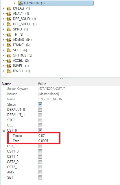
fig 5.55

After assigning the time step value, the TH is requested for springs, Parts, Accelerometers, Sections. Inorder to view the outputs, as shown in fig 5.56.

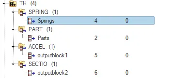
fig 5.56

Step 11: Running the simulation:-

The next step is to run the simulation. For running the simulation, the process is: Switch to analysis panel---> Select the option "Radioss"---> Save the file in some location, before running the simulation---> Click on options & enter the syntax"-nt 4" to speed up the simulation---> Click on "Radioss". It will take some time to run the simulation. After completeing the simulation, it shows a pop-up as shown in fig 5.57. Which indicates, the job is completed(i.e., Simulation is done).

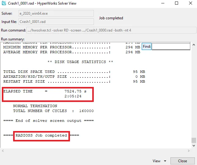
fig 5.57

The obtained animation files in the defined location appears as shown in fig 5.58.

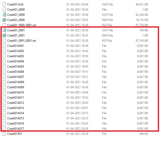
fig 5.58

Then the 0001.out file is opened. In order to view the obtained results in the form of values. The obtained results for last cycle is shown in fig 5.59.

fig 5.59

In that file at the last, the elapsed time(i.e., the time taken to complete the simulation) & the total numbar of cycles are shown in fir 5.60.

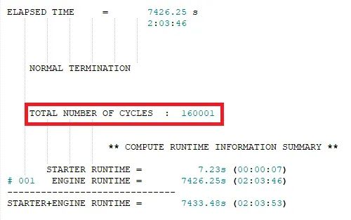
fig 5.60

Then the ontained h3d file(Combination of all animation files) is imported in another window. To view the obtained simulation. After importing it, the model with a rigid wall in the graphical display appears as shown in fig 5.61.

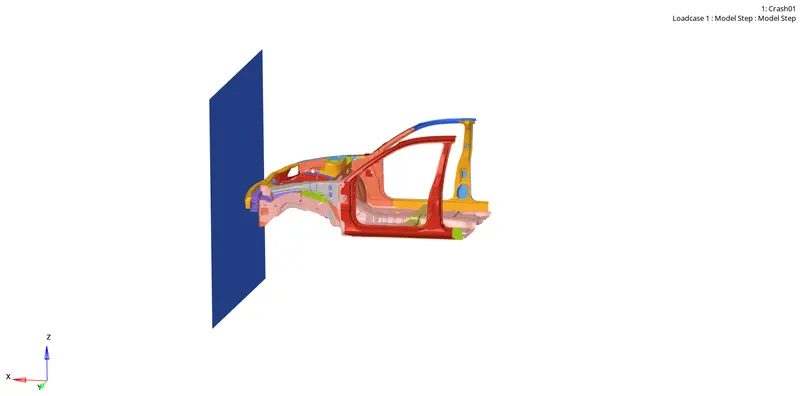
fig 5.61

Then the contour panel is opened, which appears as shown in fig 5.62. In which the parameters to view the simulation are selected. Such as: result type:In terms of Displacement, selecting the components & apply.

fig 5.62

The obtained simulation in terms of displacement is shown in the below animation.

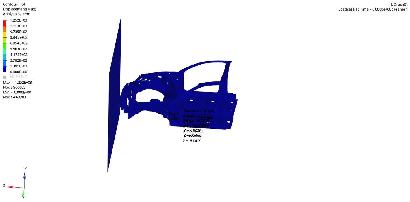
The obtained simulation in terms of mesh view is shown in the below animation.

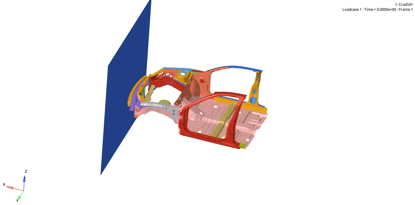
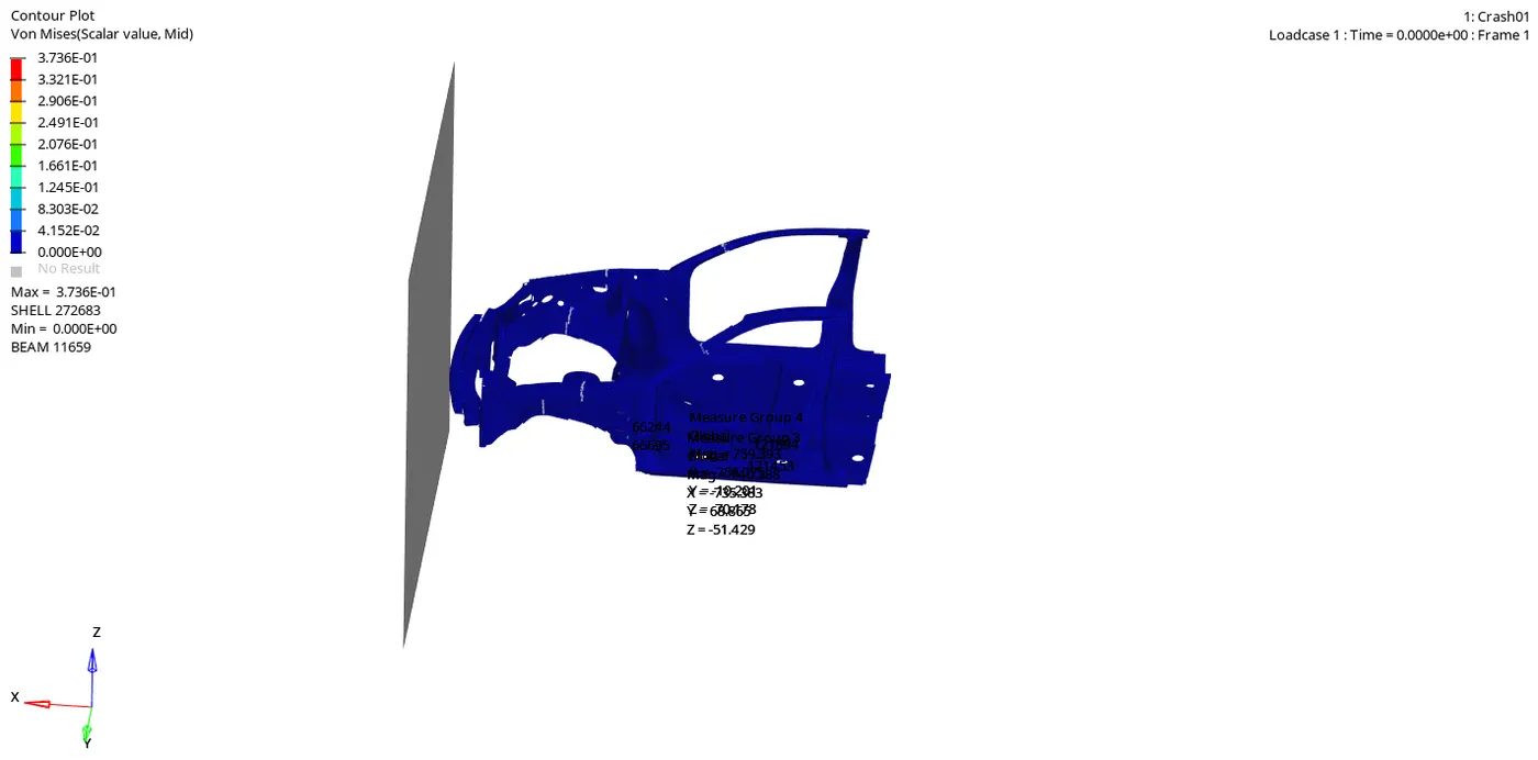
The obtained simulation in terms of Von-mises is shown in the below animation.

Step 12: Results for the intrusions:

As seen in the above animations, there are some values along the model. Those are indicated to show the intrusions. So, it can be enabled by selecting the "measures" option, as shown in fig 5.63.

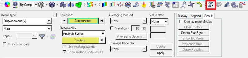
fig 5.63

After selecting that option, the nodes are to defined. After defining the nodes at the initial position(i.e., Before collision). The obtained magnitude for spring with node 66244 is 759.393 mmm & the magnitude for spring with node 66695 is 740.388 mm. As shown in fig 5.64.

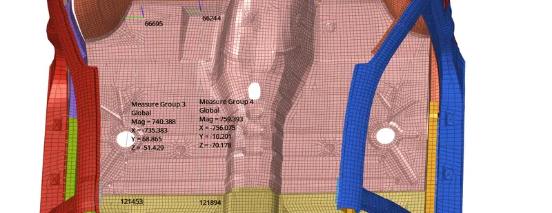
fig 5.64

Then again the deflection values are seen, as shown in fig 5.65. After the collision. The deflection value for the spring with node 66244 is 647.907 mm & the magnitude for spring with node 66695 is 664.430 mm.

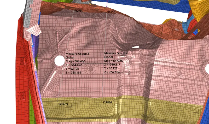
fig 5.65

The intrusions obtained in both springs are:

Spring(With node 66244) = 759.393-647.907 = 111.486 mm

Spring(With node 66695) = 740.388-664.430 = 75.958 mm

Step 13: Post-processing:-

In this step the T01 files are imported in another windows, Inorder to view the results in the form of graphs. Initially, the sectional force is plotted for the rails. The obtained graph for the left rail at the created section appears as shown in fig 5.66. With the maximum sectional force as 27.0904KN.

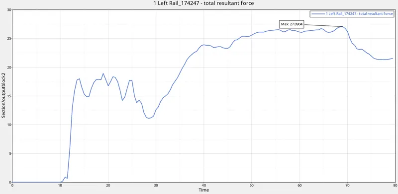
fig 5.66

The obtained graph for the right rail at the created section appears as shown in fig 5.67. With the maximum sectional force as 34.5853 KN.

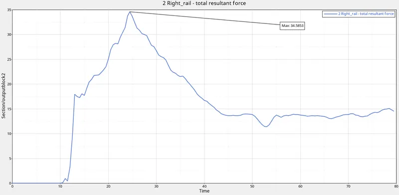
fig 5.67

Then the sectional forces are obtained for the shortgun. The obtained sectional force graph for the left shortgun is shown in fig 5.68. With the maximum sectional force as 19.7446 KN.

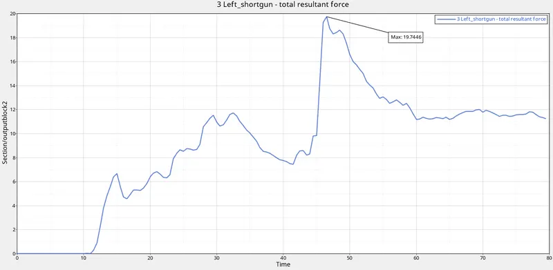
fig 5.68

The obtained sectional force graph for the right shortgun is shown in fig 5.69. With the maximum sectional force as 13.5036 KN.

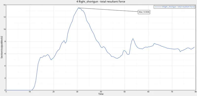
fig 5.69

Then the sectional forces are obtained for the A-pillar. The obtained sectional force graph for the left A-pillar is shown in fig 5.70. With the maximum sectional force as 3.05672 KN.

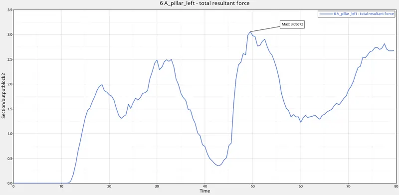
fig 5.70

The obtained sectional force graph for the right A-pillar is shown in fig 5.71. With the maximum sectional force as 2.85727 KN.

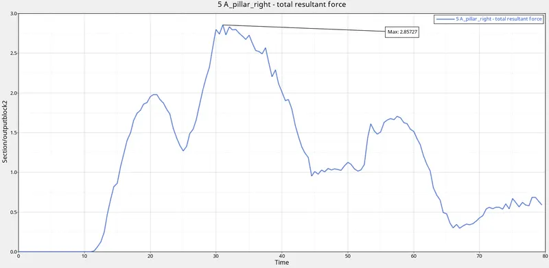
fig 5.71

Then the accelerometer graph is obtained to view the acceleration. The obtained graph for left side accelerometer appears as shown in fig 5.72. The maximum acceleration on the left side is 6.89757 m/s.

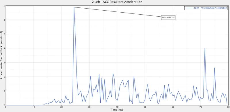
fig 5.72

The obtained graph for right side accelerometer appears as shown in fig 5.73. The maximum acceleration on the right side is 4.19141 m/s.

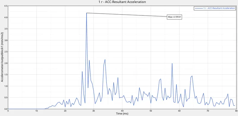
fig 5.73

Then the graphs are obtained to see the total resultant force by the interfaces. The obtained total resultant forces graph for the left bumper appears as shown in fig 5.74. With maximum force as 16.2399 KN.

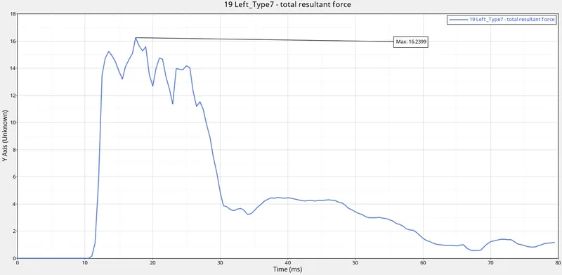
fig 5.74

The obtained total resultant forces graph for the right bumper appears as shown in fig 5.75. With maximum force as 17.3135 KN.

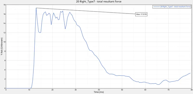
fig 5.75

The obtained total resultant forces graph for the total car( with type 7 contact) appears as shown in fig 5.76. With maximum force as 163.091 KN.

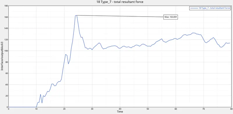
fig 5.76

Then the graphs are obtained for intrusions in two springs. The intrusion in the spring with node 66695 appears as shown in fig 5.77. With the maximum intrusion value as 75.3539 mm.

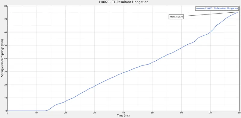
fig 5.77

The intrusion in the spring with node 66244 appears as shown in fig 5.78. With the maximum intrusion value as 110.223 mm.

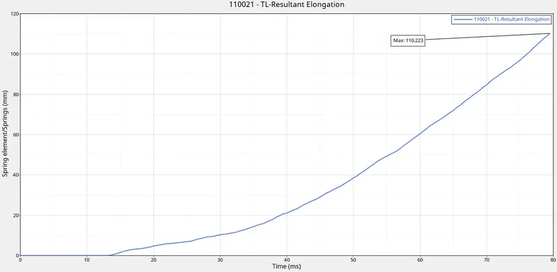
fig 5.78

Then a graph is plotted to see the variation in the sectional forces of all sections, As shown in fig 5.79.

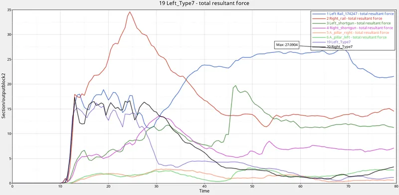
fig 5.79

From the above figure, the descending order with respect in terms of the magnitude of sectional forces & Interface forces at the bumper: Right rail, Left rail, left shortgun, Right bumper,Left bumper, Right shortgun, Left A-pillar, right A-pillar.

Finally, the energies are plotted as shown in fig 5.80. The reasons for the behavior of energies in the graph are:-

Internal energy: The internal energy will gradually increases. Because, the increase in displacement.

Kinetic energy: The kinetic energy gradually decreases. Due to the decrease in velocity. Because the given velocity is initial velocity, which may reduce.

Contact energy: The contact energy will increase slightly when the car model hits the rigid wall. Because, only some elements at the front will be having the contact.

Hourglass energy: There will be no horglass energy(i.e., constant). Because, the element formulation is specified with recommended parameters.

Total energy: There will a slight decrease in total energy. Due to the decrease in kinetic energy.

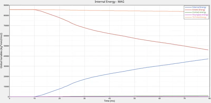
fig 5.80

6. Conclusion:

• Changed the center of gravity from initial position to the required position.
• Verified for penetrations.
• Created new interfaces.
• Created accelerometers at the base of B-pillar to obtain the acceleration.
• Assigned the initial velocity.
• Created the springs to obtain intrusions.
• Created the type 7 contact at front to obtain the axial force recieved on the rails from bumper.
• Created a rigid wall.
• Created the TH for all inputs. Inorder to obtain outputs.
• Ran the simulation.
• Finally, plotted the graphs with the obtained results(Post-processing).

7. Learning outcomes:

By performing this challenge, the following aspects can be learned:-

• Changing the COG position.
• Checking the penetrations.
• Creating interfaces.
• Creating accelerometers.
• Assigning the initial velocity.
• Creating springs to obtain intrusions.
• Creating a rigid wall.
• Requesting outputs in the form of TH.
• Verifying the obtained graphs.