Week 6 - Creating connection for Rear door

1. Objective:

• To deploy connections for the given meshed rear door model.

2. Software tool used: ANSA version 19.0.1

3. Pre-requisites:

Necesscity of connections in automotivies:

As every automobile comprises of various components & assemblies. Which should be connected by some means to withstand in space. So, there are so many techniques to deploy the connections in real world. Among them, mostly used techniques for deploying the connections in automotives are using Bolts(Temporary joint), welds(Permanent joint).

Bolted joints: Bolted joints are mainly used to resist the tension & shear between the mating parts.

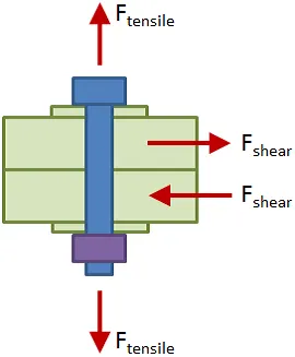
Now-a-days, the bolts are used for so many appliactions. Because of the following advantages:

• Simple operation: Bolted joints are simple joints. In bolt joint only two equipment is required bolt and nut. so this joint is simple design and operation.
• Faster joint: Welding joint and riveted joint requires more time than bolted joint. So, Bolted joint is fast in operation.
• Not permanent joint: Bolted joints are not permanent joints. So, Bolted joint is easy incase of disengagement.
• No risk: In Bolted joint, no heat is used . So, that means bolt joint is Cold process.
• No noise: Tightening bolt and nut is silent operation, When compared to the rivet joints. In riveted joints used hammer for punching of rivet. Bolted joints not required hammer so no noise is produced.
• High bolt strength: Bolt has high stength than rivet so during operation time low number of bolt required than rivet joints.

But there will be a chance of failure in some applications by using bolted joints. Some of them are:

• Insufficient Joint Clamp Force

• Bolt Thread Stripping

• Bolt Fatigue Failures

• Bolt Overload

• Excessive Bearing Stress

So, the welding joints are used to have a permanent joint betweent the components. Mostly used welding techniques in the automotives are:

• Spot welding
• Seam welding

Spot welding:

Spot welding (also known as resistance spot welding) is a resistance welding process. This welding process is used primarily for welding two or more metal sheets together by applying pressure and heat from an electric current to the weld area.

It works by contacting copper alloy electrodes to the sheet surfaces, whereby pressure and electric current are applied and heat is generated by the passage of current through resistive materials such as low carbon steels.

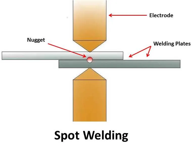
Spot welding is typically used for metal sheets with a thickness of 0.5 to 3 millimeters. And to produce the joint between the overlapping sheets.

Seam welding:

A seam weld is a continuous weld along a joint. Because the joint is forged due to the heat and pressure applied, a seam weld produces a very sturdy weld.

The fillet weld and butt joint weld are the two common types of seam welds. A fillet weld is a triangular seam weld that joins two surfaces at right angles to each other and butt welds are generally in a lap joint, T-joint or corner joint.

Unlike a spot weld that uses a single point electrode, a seam weld uses a rotating wheel electrode that produces a rolling resistance weld. This process is most often used to join two sheets of metal. MIG and TIG welders can be used to do seam welding.

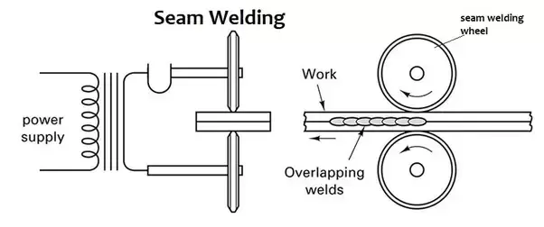
And also Seam welding is used at the load carrying regions such as joining the frames of seat etc. in automotives.

So, to permorm any analysis such as crash, NVH, durability. The components should be connected. So, these are represented virtually in the software. Which will be seen in the procedure.

In some regions the rigid elements such as RBE2 & RBE3 are used, Inorder to possess the rigid nature.

4. Procedure:

Initially, the given rear door model should be imported in to the ANSA software. After importing, the given model appears in the graphical display as shown in fig 4.1

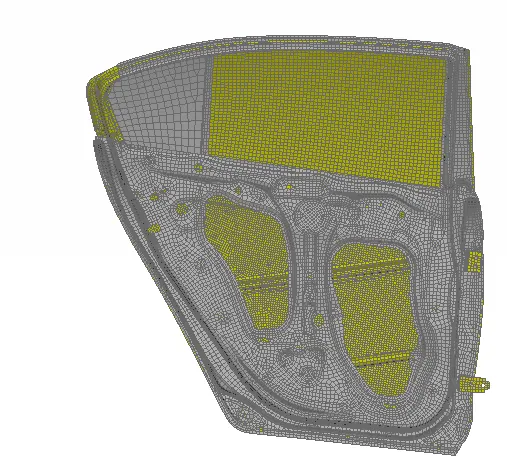
fig 4.1

Then the given model is viewed in the PID form. By choosing PID view, the entire model appears to be in a same PID. with the same colour, as shown in fig 4.2.

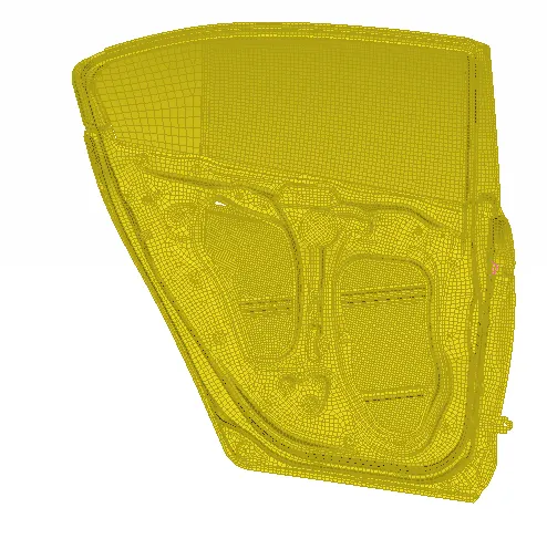
fig 4.2

To deploy the connections, the entire model should be seperated in to some PID's. Based on the components, the entire model is seperated and it will be named in the data base window. As shown in fig 4.3.

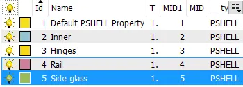
fig 4.3

The connections are deployed at different regions.

Step 1: Deploying the Connections at Hinges:

Initially, the connections are deployed at the hinge regions. Which connects the door sub-system and the body of the car. The hinge region appears as shown in fig 4.4.

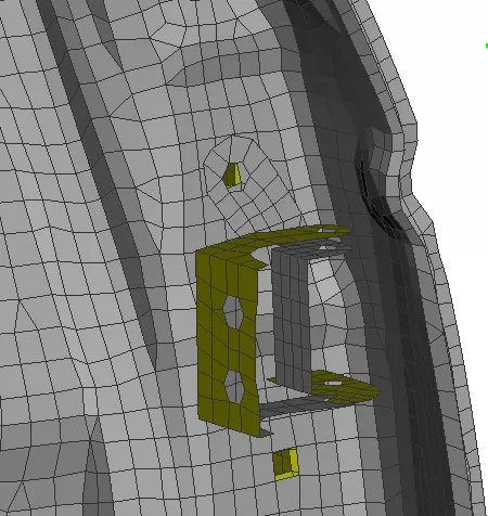
fig 4.4

At the hinges, the bolted joint is used in the real scenario. So to replicate that virtually, the bolted joint is created. For creating a bolt connection, A COG point is required. Which is available in "Points" from "Topo" module, as shown in fig 4.5.

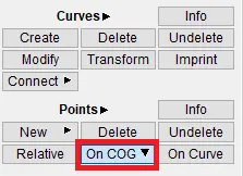
fig 4.5

After selecting the COG option, any one of the closed perimeter should be selected as shown in fig 4.6.

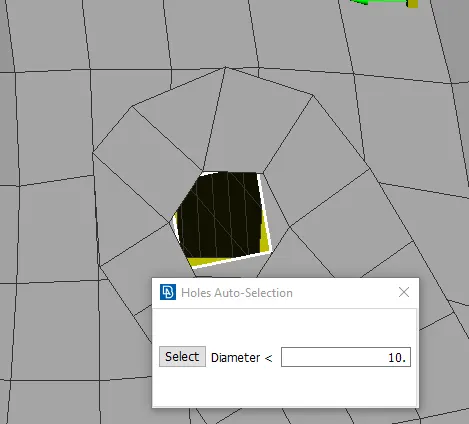
fig 4.6

After selecting the closed perimeter by middle clicking on the mouse, the COG point of that perimeter will be generated. Which is represented as a square with the sky-blue colour, as shown in fig 4.7.

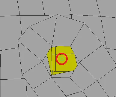
fig 4.7

Then the created COG point should be converted to a 3D point from the "Convert" option in assembly manager. As shown in fig 4.8.

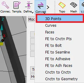
fig 4.8

Then the 3D point should be selected and bolt option should be selected. Inorder to convert the 3D point to bolt. As shown in fig 4.9.

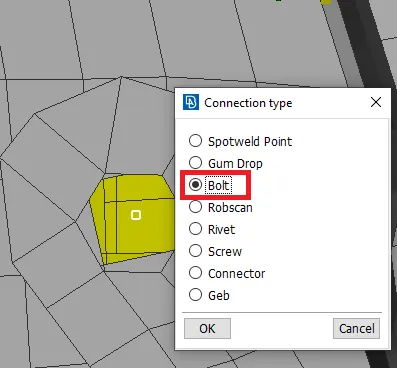
fig 4.9

After converting the 3D point to bolt, the bolt will be represented as hexagonal shaped bolt. As shown in fig 4.10.

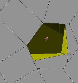
fig 4.10

Then by using "connection" option from the assembly manager, the bolt should be selected. The dialog box appears, as shown in fig 4.11.

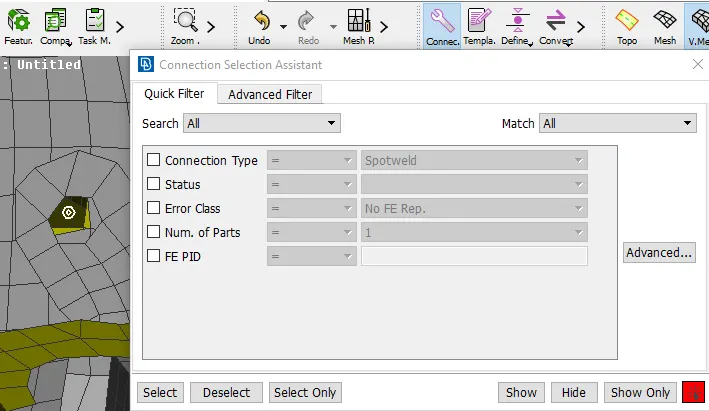
fig 4.11

Then by middle clicking, a dialog box appears as shown in fig 4.12. Which represents the connection manager. In which some parameters such as PID 1, PID 2, FE representation type should be selected. Then by selecting Apply, Realize the connection will be realized.

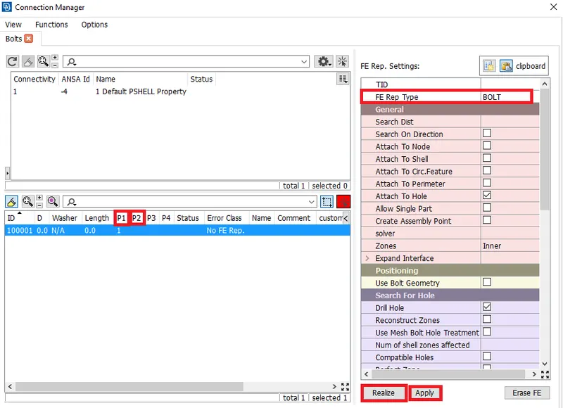
fig 4.12

After realizing the connection, the formed bolt connection with the bolt stem appears as shown in fig 4.13.

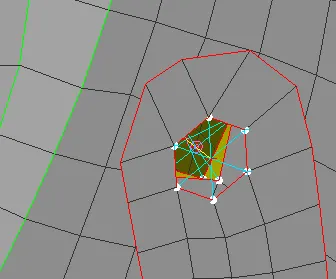
fig 4.13

Then the connection is deployed using RBE2 cluster in some regions as shown in fig 4.14. In which the RBE2 element---> Many nodes option should be selected. RBE2 cluster means, connecting so many nodes.

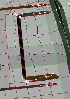
fig 4.14

Then a RBE2 element, with two nodes option in the NASTRAN deck module is choosed. As shown in fig 4.15. Inorder to connect the created RBE2 cluster.

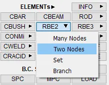
fig 4.15

After selecting the two nodes(i.e., Master nodes of the created RBE2 cluster), a dialog box appears as shown in fig 4.16. WHich represents the info about RBE2 elements. In which CM(Degrees of freedom) should be constrained in all directions except rotation in Z-direction(i.e., enabling CM only in 1,2,3,4,5). Because, the door will be moved in rotation with respect to Z-axis.

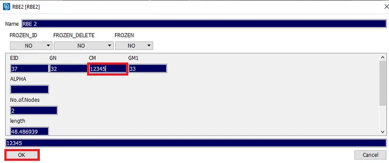
fig 4.16

By clicking "Ok" , the RBE2 element with 2 nodes is created in between two RBE2 cluster elements. Which is represented by a "Yellow" coloured line. As shown in fig 4.17.

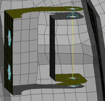
fig 4.17

Step 2: Deploying the connections with RBE2 elements:

Similarly, the RBE2 elements are deployed at some regions. With many nodes option. As shown in fig 4.18.

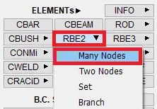
fig 4.18

After selecting the many nodes option, The nodes should be selected as shown in fig 4.19. After selecting the nodes, by clicking on "Next" the slave nodes will be selected.

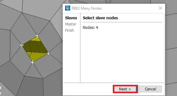
fig 4.19

After selecting "Next", a dialog box appears as shown in fig 4.20. Which represents the method to create a master node. And the preview of the master node is also shown in the red colour.

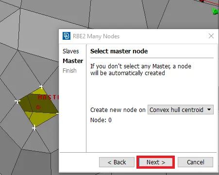
fig 4.20

Then by clicking "Next", a RBE2 element will be created as shown in fig 4.21. And also it shows the information regarding the created RBE2 element in a dialog box. By clciking "Finish", the connection will be realized completely .

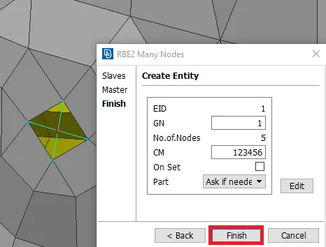
fig 4.21

The created RBE2 links can be seen in the model browser. As shown in fig 4.22.

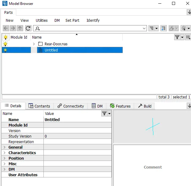
fig 4.22

Similarly, the rigid(RBE2) elements are used to connect various PID's where the parts should be rigid enough at the time of simulation. After deploying the connections with RBE2 elements through out the model, the model with RBE2 elements appears as shown in fig 4.23.

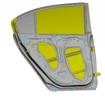
fig 4.23

Step 3: Deploying a connection at the door handle:

Then the connection is deployed at the door handle region. Which is shown in fig 4.24.

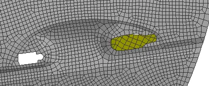
fig 4.24

Initially, the RBE2 elements with many nodes option is used to connect all nodes at the perimeter of the handle. As shown in fig 4.25. Inoder to possess the rigid nature.

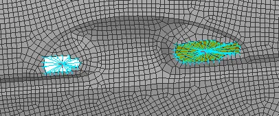
fig 4.25

Then a RBE2 element with many nodes is used to connect the both master nodes. After connecting, it appears as shown in fig 4.26.

Note: The reason behind using RBE2 with many nodes rather than RBE2 with two nodes is, to have a master node after connecting those two master nodes. But in case of RBE2 with two nodes, there will be no master node after connecting those two portions.

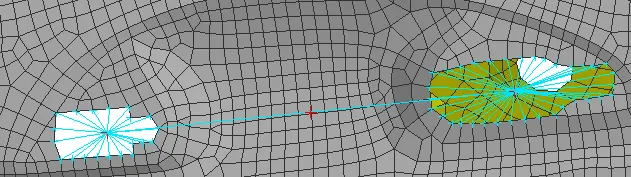
fig 4.26

Then to represent the weight of the door handle, as in case of real world scenario. The mass can be assigned by using the "CONMi" ---> CONM2---> Nodes. In NASTRAN deck module, as shown in fig 4.27.

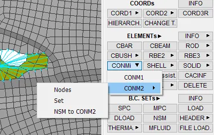
fig 4.27

A weight is assumed as 1 kg and entered as "1e-4"(Which will be in the form tonns). As shown in fig 4.28. And this is applied to the master node at the center.

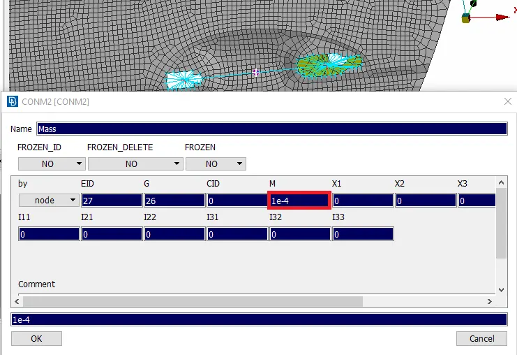
fig 4.28

After assigning the mass at the center master node, it will be represented as highlighted one as shown in fig 4.29.

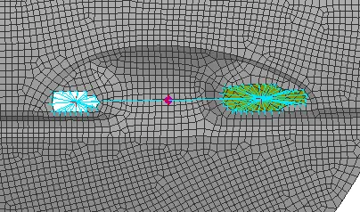
fig 4.29

Step 4: Deploying a Connection at the latch region:

As the latch is the part which is responsible for opening the door, it is connected by using the RBE2 element with many nodes to form a cluster. As shown in fig 4.30

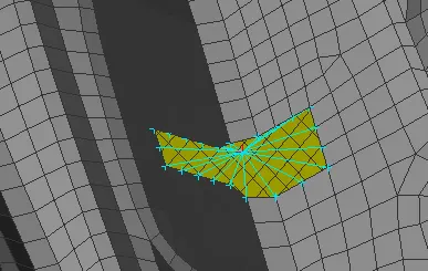
fig 4.30

Step 5: Deploying a Connection between the rail & side glass:

In this step, the rail which is responsible for the movement of side glass to up & down and the side glass are only isolated to have a clarity on them. As shown in fig 4.31.

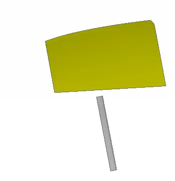
fig 4.31

By isolating those components the thing noticed is, the rail component should be enlarged a bit more till the glass. This can be done by using "Move free" option in grids from mesh module. As shownin fig 4.32. And the nodes at the edges are selected to enlarge in z-direction.

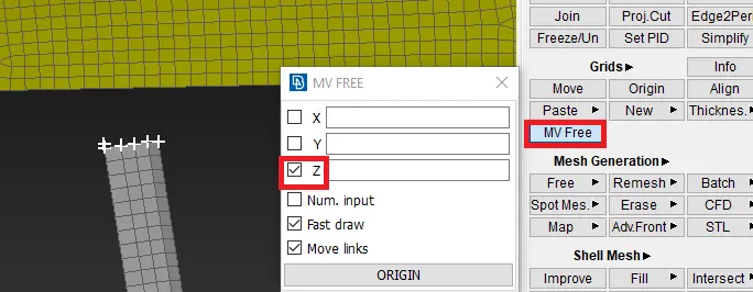
fig 4.32

After enlargment, it appears as shown in fig 4.33.

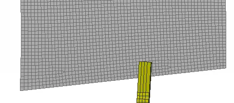
fig 4.33

But the enlarged elements will be too high interms of length. So, those elements are selected and reconsturtion of elements is performed. By assigning the target element length, as by measuring any one element dimensions. As shown in fig 4.34.

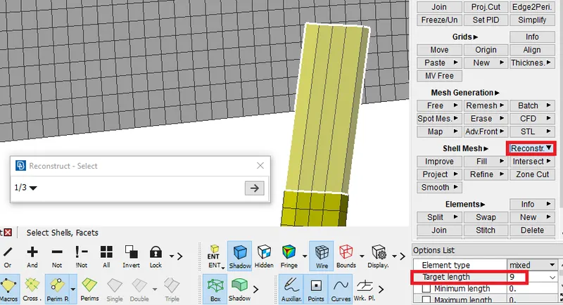
fig 4.34

After performing reconstruction, the rail component appears as shown in fig 4.35.

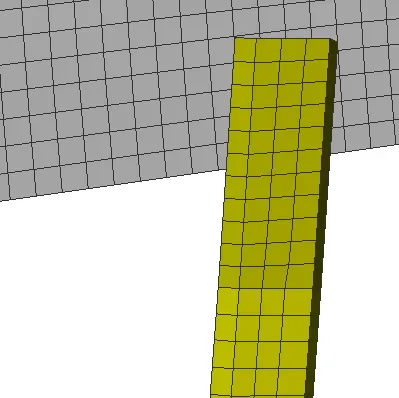
fig 4.35

These two components are connected by using RBE2 elements. To possess rigid nature. So for proper selection of entities, the elements option is enabled. As shown in fig 4.36. Which indicates the entities selected will be elements.

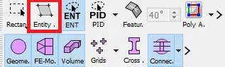
fig 4.36

After selecting the elements and confirmed the connection, the connection is deployed by a RBE2 cluster element between rail & glass. As shown in fig 4.37.

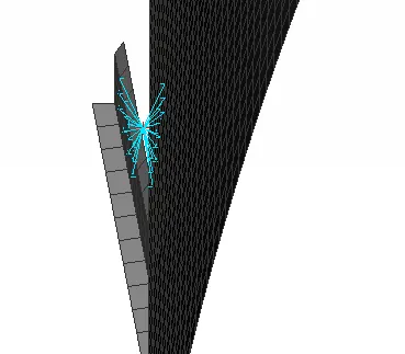
fig 4.37

Step 6: Deploying the connections using spot weld:

In some regions where the parts overlaped with each other with the minimal space between them are joined using spot weld option. In order to represent the joint. So for creating a spot weld connection, the COG point is required. And the edges of the element is selected by choosing the "on COG" option as shown in fig 4.38.

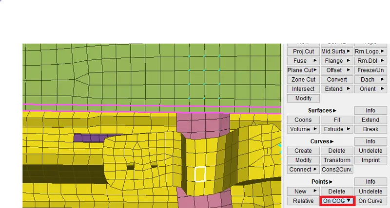
fig 4.38

AFter craeting a COG point, it is converted to a spot weld point. This done by choosing, "Convert" option from assembly manager. And in that, the connection type is specified as "spot weld point". As shown in fig 4.39.

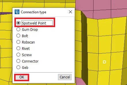
fig 4.39

Then to realize this connection, the connection manager is opened from assembly manager. And the converted spot weld point is selected. And some parameters are specified as shown in fig 4.40. And the FE reresentation of a spot weld connection in NASTRAN deck is "RBE3-HEXA-RBE3".

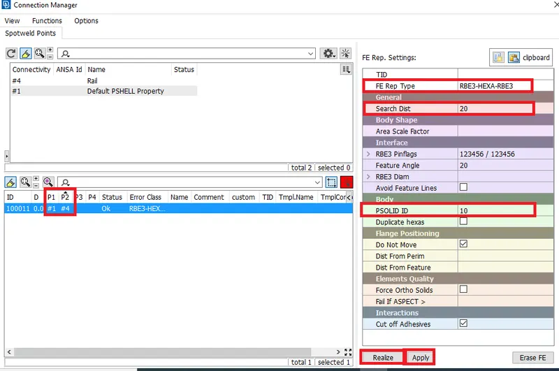
fig 4.40

After realizing the connection, it appears as shown in fig 4.41. SImilarly, the spot weld connection is deployed. Wherever it is necesscary.

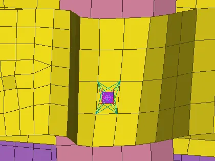
fig 4.41

Step 7: Deploying the connections at the side glass region:

As the side glass is surrounded by a component called "Weather strip" which is made up of rubber material. And widely known as "Beading". So to represent that, the CBUSH elements are used. Because, it possess the elasticity in all three directions.

So, initially the curves are needed. For that, the "FEA to curve" option in the perimeters from topo module is used. Which is shown in fig 4.42.

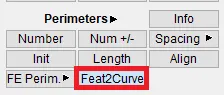
fig 4.42

And the FEA edges are selected one by one and then it is converted in to curves, which are represented by purple coloured lines at the edges. As shown in fig 4.43.

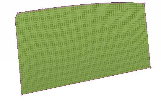
fig 4.43

As the weather strips will be at the both sides of the glass at the bottom, the CBUSH elements should be deployed at the both sides of bottom. For doing that, the curve created at the bottom should be copied by using "Transform" and moved to a certain distance such as 10mm. As shown in fig 4.44.

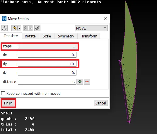
fig 4.44

After copying & moving, the moved curve appears as shown in fig 4.45.

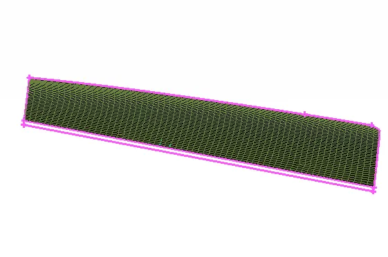
fig 4.45

Then these curves are converted in to "spot line". And then this spot line is realized by selecting the line by line and specifying the parameters such as spacing between the CBUSH elements as 10 mm, specifying PART1 & PART 2, specifying FE represntstion type as "RBE3-CBUSH-RBE3" and assigning RBE3 pinflags(DOF) in all directions. As shown in fig 4.46.

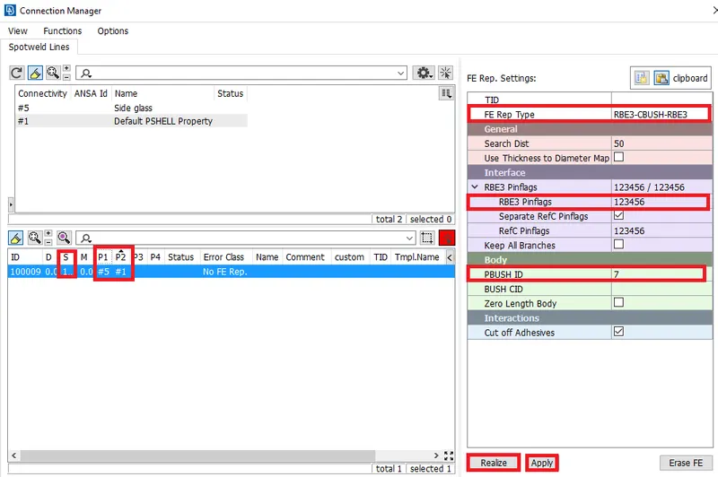
fig 4.46

Then the PID should be created, which is done by selecting "Shift+?" from key-board by placing the cursor in the PBUSH ID row of fig 4.46. After selecting a "new" option, a diaog box appears as shown in fig 4.47. WHich represents to PID for the CBUSH elements. In that, the 6 stiffness values are entered, which are predfined.

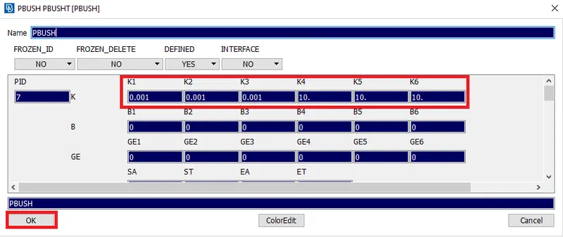
fig 4.47

After creating the new PID for CBUSH elements, the CBUSH elements will be formed in between the side glass and outer part. As shown in fig 4.48.

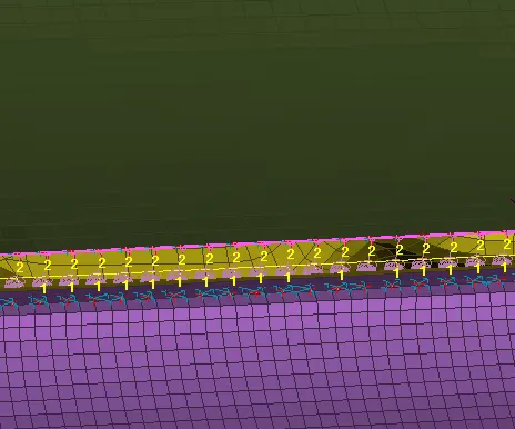
fig 4.48

Similarly, the CBUSH elements are created on all sides of the glass. Then the created CBUSH elements are isolated. After isolating them the thing noticed is, the CBUSH elements are in different orientations. As shown in fig 4.49. Which may lead to the in appropriate results at the time of simulation.

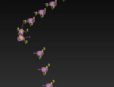
fig 4.49

So to overcome that problem, the orientation of all CBUSH elements should be changed to that of global co-ordinate system, For doing that, all of the CBUSH elements are enabled from the data base window. As shown in fig 4.50.

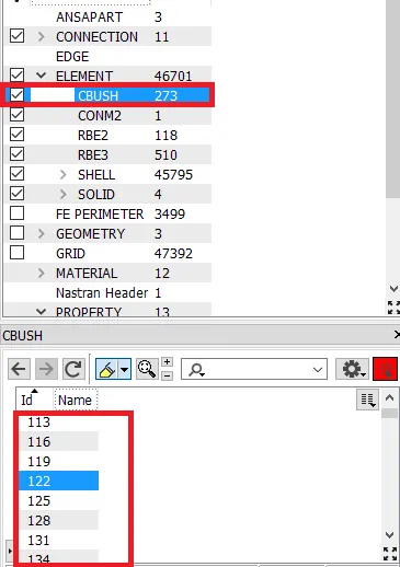
fig 4.50

Initially, any one of the element is selected and the orientaion is choosed to "With Cord", which means "With respect to co-ordinate axis. And the CID is given as "0", As shown in fig 4.51. which depicts that, the orientaion with respect to global co-ordinates.

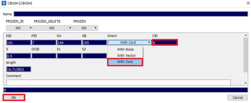
fig 4.51

By isolating only that CBUSH element, the co-ordinates of that element will be changed to same as that of global co-ordinates. As shown in fig 4.52.

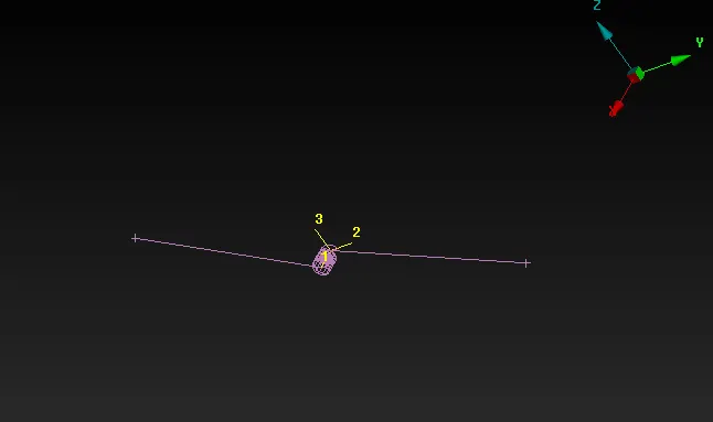
fig 4.52

So for doing the same to all CBUSH elements, they are enabled. And by selecting the drop down box which is highlighted in fig 4.53. The list fields to be included with the elements are shown. In that, CID & orientation are enabled. Thereby select the "modify" option in that CID region.

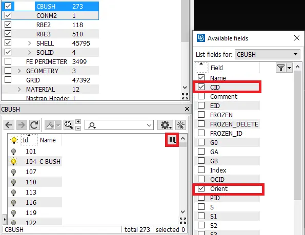
fig 4.53

Then by clicking "Ok", a dialog box appears as shown in fig 4.54. Which indicates the selection of CID(Co-ordinate ID) for all elements. And the values are specified, as shown in fig 4.54.

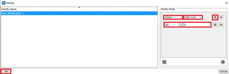
fig 4.54

By clicking "Ok", a dialog box appears as shown in fig 4.55. Which depicts a warning message by indicating that the change in CID is ok to continue or not.

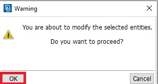
fig 4.55

After clicking "Ok", all CBUSH elements will be in same orientation. As shown in fig 4.56.

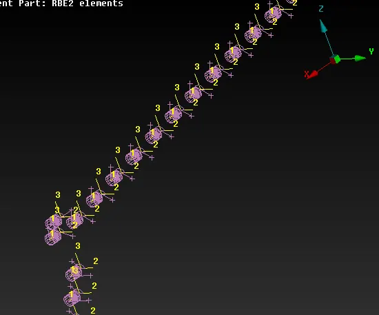
fig 4.56

Finally after deploying all necesscary connections to the given rear door model, it appears as shown in fig 4.57.

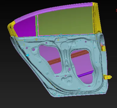
fig 4.57

5. Conclusion:

• Finally, Deployed the necesscary connections for the given meshed rear door model.

6. Learning outcomes:

By performing this challenge, the following aspect can be learned:

• Deploying connections using rigid (RBE2) elements in ANSA.
• Deploying connections using Bolt joints in ANSA.
• Deploying connections using CBUSH elements in ANSA.
• Applying the mass to a node(At the door handle).
• Assigning the Degrees of freedom for the created elements.
• Changing the orientations of CBUSH elements.