Week 3 - Solving second order ODEs

Objective:

• To write a code for determining the change in position of a pendulum by using an ordinary differential equation(ODE)(with the second order differential equation).
• To obtain a plot which depicts the change in angular velocity & displacement with respect to time.
• To create a animation file showing, how the simple pendulum moves as a function of time.

Software tool used: MATLAB R2021a

Procedure:

Initially, after opening the MATLAB software tool, the pre-requisite commands such as clear all, close all, clc are entered & the inputs required(such as Length of the pendulum, Mass of the ball, Damping coefficient & Acceleration due to gravity) to define the given second order differential equation are entered. Which appears as shown below.

clear all 
close all
clc

% Inputs:
  
L = 1           % Length of the pendulum in meters.

m = 1           % Mass of the ball in kg.

b = 0.05        % Damping coefficient.

g = 9.81        % Acceleration due to gravity in m/s^2.

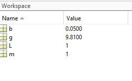
After entering the inputs, the code is runned. Inorder to check for assigning the variables with the values. After successful running of the code, the variables assigned with values appears in the work space window, as shown in below fig.

Then the initial conditions of the problem(Pendulum at rest) are defined. An array is created with the variable named "Theta_0". Which consists of Angular diaplacement as 0 metres & Angular velocity as 3 rad/sec. As shown below.

And the problem is integrated by assigning the time points form 0 to 20 seconds by using "linspace" command. As shown below.

Linspace command syntax: linspace(starting point, Ending point, No of outputs required in between the starting & ending points with the same interval).

% Initial condition:
Theta_0 = [0;3];    % Where at time t = 0, The given Angular displacement = 0 m, Angular velocity = 3rad/sec.


% Time points(Integrating the system from 0 to 20 seconds):
T_span = linspace(0,20,500);

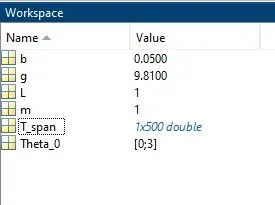
Then the code is runned. After running the code, the obtained output for given time points, Angular diaplacement & Angular velocity are assigned to the given variables in the work space window. As shown in below fig.

Then a syntax is used to solve the given ODE. Which appears as the code shown below.

% solution step:
[t, results] = ode45(@(t,Theta) ode_func(t, Theta, b, g, L, m), T_span, Theta_0);

In which, ode45 ----> Pre-defined solver in MATLAB.

(t, Theta) ---> Main inputs for the ODE, Which are the dependent & independent variables of the ODE system.

ode_func(t,Theta, b,g,L,m) ---> ODE function definition which is already written as another code. Where b,g,L,m are inputs.

T_span ---> Time integration

Theta_0 ---> Initial conditions

The "ode-func" is a separate code written. which appears as shown below.

function [dTheta_dt] = ode_func(t, Theta, b,g,L,m)
Theta1 = Theta(1);
Theta2 = Theta(2);
dTheta1_dt = Theta2;
dTheta2_dt = -(b/m)*Theta2-(g/L)*sin(Theta1);
dTheta_dt = [dTheta1_dt; dTheta2_dt];

end

Which involves converting the second order ODE to a single order ODE's. The significance of converting them is, to bring down the complexity of the problem.

Conversion of the second order ODE to a single order ODE's:

Given second order ODE: [d^2(`Theta`)/dt^2] +[b/m*d(`Theta`)/dt]+[g/l*sin`Theta`] =0 ----> eq(1)

Inorder to convert this, Two assumptions are made. Which are: `Theta` = `Theta`1

d(`Theta`)/dt = d(`Theta`1)/dt = `Theta`2 ----> First ODE

Then by substituting this in eq(1) ---> [d^2(`Theta`1)/dt^2] +[b/m*d(`Theta`1)/dt]+[g/l*sin`Theta`1] =0

---> [d/dt(`Theta`2)]+[(b/m)*`Theta`2]+[(g/L)*sin(`Theta`1)] =0

---> d(`Theta`2)/dt =`-[(b)/(m)``Theta`2]-[`g/L`*sin`Theta`1]---> Second ODE

Then these are combined as an array, with the variable named: d`Theta`/dt. Which is mentioned as: dTheta_dt in the last line of the above code.

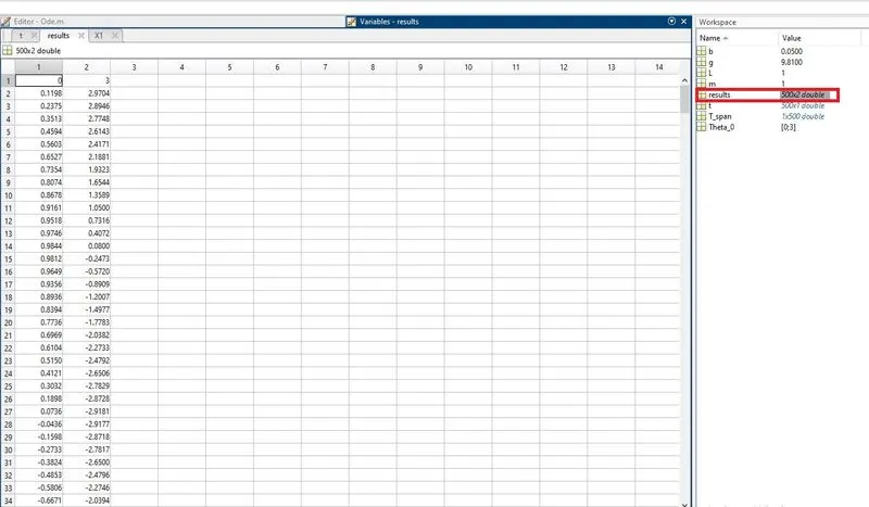
Then the code is runned, the outputs are stored in a variable named "results" in the work space window. Which consists of 500 rows & 2 columns. In which the values in the first column represents the values of angular displacement & second column represents the values of angular velocity(Which starts from 3rad/sec). As shown in below fig.

Then the obtained results are plotted in graph, by using "plot" command. As shown in the code below.

% Results(In terms of plot):
figure(1)
plot(t, results(:,1),'color','b')
hold on
plot(t, results(:,2),'color','r')
xlabel('Time(seconds)')
ylabel('Angular Velocity(m/sec) & Displacement(m)')
legend('change in Displacement', 'change in Angular veloctiy')
hold off

The significance of the above steps are:

figure(1) ---->Starting a new plot with the name as "figure(1)".
plot(t, results(:,1),'color','b') ---> To plot the results in terms of time & obtained values in first column(i.e., values associated with Angular displacement).

hold on ----> To hold the actions of previous plot.
plot(t, results(:,2),'color','r') ---> To plot the results in terms of time & obtained values in secondcolumn(i.e., values associated with Angular velocity).
xlabel('Time(seconds)') ---> To name the X-axis as "Time in seconds".
ylabel('Angular Velocity(m/sec) & Displacement(m)') ----> To name the X-axis as "Angular Velocity in metres/sec & Displacement in metres".
legend('change in Displacement', 'change in Angular veloctiy') ---> To distinguish the obtained plots in terms of colors.
hold off ---> To stop holding the actions till now in figure 1.

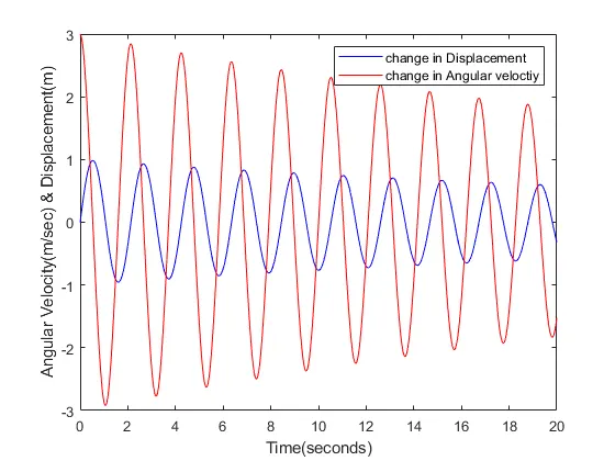
Then the code is runned. After running the code, the obtained output in terms of plot appears as shown in below fig.

Obtaining the animation for pendulum:

Then, the code is written for obtaining an animation file. Which appears as shown below.

% Animation

ctr = 1
for i = 1: length(results(:,1))
    
    % Inputs:
    X0 = 0;
    Y0 = 0;
    
figure(2)
    X1 = L*sin(results(i,1));
    Y1 = -L*cos(results(i,1));
    plot([-1,1],[0,0],'linewidth',4,'color','B')

Where, The significance of those steps are as follows:

ctr = 1 ---> Introducing a counter command. To perform the loop, which starts from 1.
for i = 1: length(results(:,1)) ---> Introducing a for loop, for performing the repetitive tasks with a variable named "i". Which performs the tasks from 1 to entire values of the obtained results(All rows, first column).

% Inputs:
X0 = 0;
Y0 = 0; ---> Co-ordinates of the pendulum at rest(or) at initial stage.
figure(2) ---> Starting another plot with the name as "figure(2)".
X1 = L*sin(results(i,1)); ---> Changing position of a pendulum for all iterations of angular displacement interms of X co-ordinate.
Y1 = -L*cos(results(i,1)); ---> Changing position of a pendulum for all iterations of angular displacement interms of Y co-ordinate.
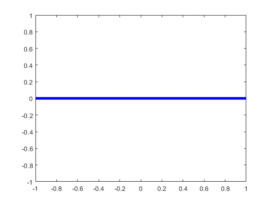
plot([-1,1],[0,0],'linewidth',4,'color','B') ---> To plot the fixed end of pendulum with the axis of X:[-1 to 1] & Y: [0, 0]. with a line width of 4(To have a thick line). Represnting with "Blue" color.

Then the code is runned. After running the code, the obtained fixed end appears in the plot as shown in below fig.

Then the further commands are entered as shown below. Inorder to represent the pendulum & bob. As shown below.

 hold on
    plot([X0 X1],[Y0 Y1],'color','b')
    hold on
    plot(X1, Y1, '.','markersize',50)
    grid on
    axis([-2 2 -2 2])
    pause(0.03)
    hold off
    M(ctr) = getframe(gcf)
    ctr = ctr+1
  
end

Where, The significance of those steps are as follows:

hold on ---> To hold the actions of previous plot.
plot([X0 X1],[Y0 Y1],'color','b') ---> To plot the change in the positions of pendulum with X cordinates from X0 to X1 & Y coordinates from Y0 to Y1 with blue coloured line representation.
hold on ---> To hold the actions of previous plot.
plot(X1, Y1, '.','markersize',50) ---> To represent the "Bob", as a dot with the size of 50.
grid on ---> To switch on the gird.
axis([-2 2 -2 2]) ---> To switch on the axis for representation of X-axis from -2 to 2 & Y-axis from -2 to 2.
pause(0.03) ---> To pause the code for some time. Inorder to have a proper identification of the changes in position of pendulum.
hold off ---> To stop holding the actions till now in figure 2.
M(ctr) = getframe(gcf) ---> Storing the changes in position of pendulum in a variable named "M" with the help of "counter" command.
ctr = ctr+1 ---> Iterations for the counter command.
end ---> Indicates the end of for loop.

Then the commands shown below are written to stitch all images in the form of a video.

movie(M)
videofile = VideoWriter('pendulum_ode.avi')
open(videofile)
writeVideo(videofile,M)
close(videofile)

After writing those commands, the program is runned. After running the program, the output in the form of an animation file appears as shown in below link.

https://youtu.be/osHjj0VSWJg

Results:

The final code for determining the change in position of a pendulum by using an ordinary differential equation(ODE)(with the second order differential equation) appears as shown below.

clear all 
close all
clc

% Inputs:
  
L = 1           % Length of the pendulum in meters.

m = 1           % Mass of the ball in kg.

b = 0.05        % Damping coefficient.

g = 9.81        % Acceleration due to gravity in m/s^2.

% Initial condition:
Theta_0 = [0;3];    % Where at time t = 0, The given Angular displacement = 0 m, Angular velocity = 3rad/sec.


% Time points(Integrating the system from 0 to 20 seconds):
T_span = linspace(0,20,500);

% solution step:
[t, results] = ode45(@(t,Theta) ode_func(t, Theta, b, g, L, m), T_span, Theta_0);

% Results(In terms of plot):
figure(1)
plot(t, results(:,1),'color','b')
hold on
plot(t, results(:,2),'color','r')
xlabel('Time(seconds)')
ylabel('Angular Velocity(m/sec) & Displacement(m)')
legend('change in Displacement', 'change in Angular veloctiy')
hold off


% Animation

ctr = 1
for i = 1: length(results(:,1))
    
    % Inputs:
    X0 = 0;
    Y0 = 0;
    
figure(2)
    X1 = L*sin(results(i,1));
    Y1 = -L*cos(results(i,1));
    plot([-1,1],[0,0],'linewidth',4,'color','B')
    hold on
    plot([X0 X1],[Y0 Y1],'color','b')
    hold on
    plot(X1, Y1, '.','markersize',50)
    grid on
    axis([-2 2 -2 2])
    pause(0.03)
    hold off
    M(ctr) = getframe(gcf)
    ctr = ctr+1
  
end

movie(M)
videofile = VideoWriter('pendulum_ode.avi')
open(videofile)
writeVideo(videofile,M)
close(videofile)

The final plot with "Time" Vs " Angular velocity & displacement" appears as shown in below fig.

The final output in the form of an animation file for the change in position of a pendulum as a function of time appears as shown in below link.

https://youtu.be/osHjj0VSWJg

Conclusion:

• Written a code for determining the change in position of a pendulum by using an ordinary differential equation(ODE)(with the second order differential equation).
• Obtained a plot which depicts the change in angular velocity & displacement with respect to time.
• Finally, Created an animation file showing the simple pendulum moves as a function of time.