Assignment 2-RADIOSS Engine File Editing & 3D Meshing Challenge
1. To find: Speed of sound in steel rail(C):-
Formula used: C = `sqrt(E/rho)`
Where: "E" is Young's modulus (Which is the ratio of stress and strain with in the elastic limit) SI unit for it is "Pascal (Pa)".
1 Pa = 1*1o^-6 N/mm^2 (1Mpa= 10^6 Pa, 1GPa=10^9Pa), For steel E = 2.1*10^5 N/m^2 (or) Pa.
"rho" is the density of the material. SI unit of it is "Kg/m^3".
1 Kg/m^3 = 0.001 g/cc=0.001g/cm^3, For steel rho = 0.0078 g/mm^3
Now, C = 2.1*10^5/0.0078
= 5188.74 m/s
Therfore, speed of sound in steel rail is 5188.74 m/s
2. Given data: Length of rail = 1000 mm
To find: Time taken by a shock wave to travel from one end of the rail to the other end:-
Formula used: Speed = Distance`-:` Time
SI unit of distance is "Meter (m)", ( 1m = 100 cm= 1000 mm)
SI unit of time is "Second(s)"
SI unit of speed is "Meter(m)`-:`Second(s), 1m/s= 18`-:`5 Km/hr (or) 3.6 Km/hr
Now, Time(t)= Distance`-:`Speed = 1000`-:`5188.74
= 0.1927s
Therefore, the time required for a shock wave to travel from one end of the rail to the other end of the rail is 0.1927s
3. To find: Time for sound to travel length of rail:-
Time for sound to to travel through out the length of rail = Time taken by a shock wave to travel from one end of the rail to the other end
= 0.1927s
Therefore, the time required for sound to travel the entire span of rail is 0.1927s
4. To edit the engine file so that the stress wave can be monitored, moving from one end of the rail to the other during impact, Which requires a termination time equal to the time it takes for the sound to travel the length of the rail:-
Any model in radioss solver,for analysis will have two files. They are:
- Starter file
- Engine file
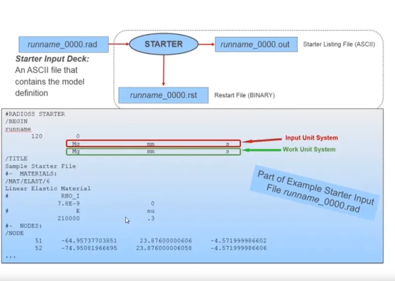
Starter file: Starter file is a file, that consists of the entire model information such as nodes information, mesh information, load definitions, boundary conditions, material laws, contact details. It is also known as "Input Deck". It is represented by "runname_0000.rad".
Where runname is the name through which the file saved. It depends on the user.
0000.rad is the syntax of the starter file. It can not be changed. Starter input deck consists of multiple input blocks. Each input block starts with '/' and ends with the beginning of each block.A sample starter file is shown in the below figure.
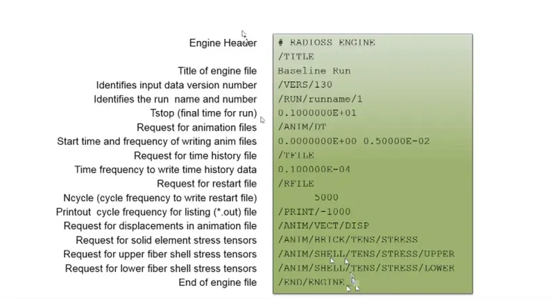
Engine file: Engine file is a file, that contains the running instrucions for the solver. It also contains animation outputs expected from the model. The engine input file is represented as "runname_0001.rad". Where 0001.rad is the syntax of the engine file. A sample of engine file is shown in the below figure.
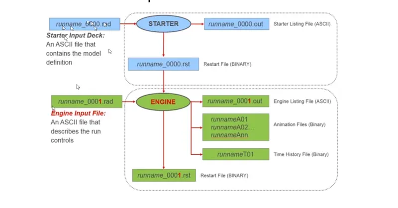
Starter, engine and output files are of ASCII file type. Which will be in the form of a code and human readable. Where as, the other files such as restart, time history, animation files are of Binary file type. Which will be in the form of 0 & 1 and are not readable by human.
Note: Both starter & engine files should have the same file name.
The block diagram of a radioss input files is shown in below figure.
Procedure for editing the engine file:
Initially, the given starter file is imported in the hyperworks with radioss as user profile. This is done by clicking on "Import" option. After doing that, "Import solver deck" shold be selected as shown in fig 4.1
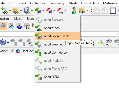
fig 4.1
Then the file selection panel opens as sshown in fig 4.2. In that the file type (Radioss), file shoud be selected properly. And then by clicking on import, The file will be imported.
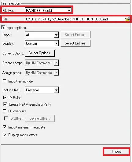
fig 4.2
The imported model appears in the grahical display as shown in fig 4.3.
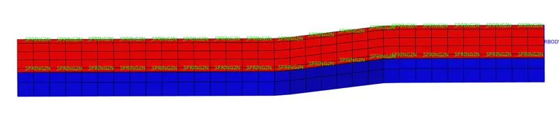
fig 4.3
After getting the model, there will be cards assigned to the model. In which the values to be edited. The cards appears as shown in fig 4.4.
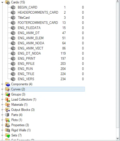
fig 4.4
Now, the values obtained in the above questions are entered in to that respective cards. As we got the T frequency value as 0.009635, This value is entered in the parameter named Tfreq in the card named "ENG_ANIM_DT" as shown in fig 4.5.
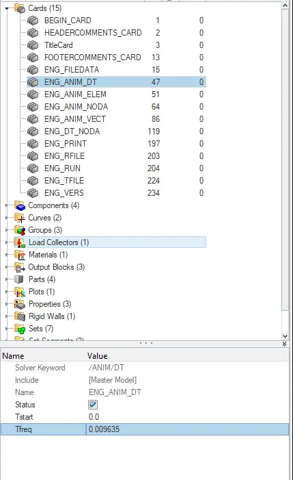
fig 4.5
Then the obtained time step value is entered in the card named "ENG_RUN" as shown in fig 4.6.
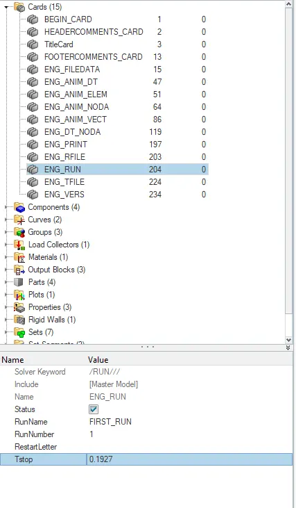
fig 4.6
Then by clicking on "Analysis" panel from main menu page. The analysis panel appears as shown in fig 4.7. Cilck on the radioss option.

fig 4.7
After opening the radioss, Initially the file should be saved in a folder. Then by clicking on the Radioss again as shown in fig 4.8. The solver will run simulation in the back end.

fig 4.8
After completing the work, radioss will send a pop-up. Indicating that, the radioss job is completed as shown in fig 4.9.
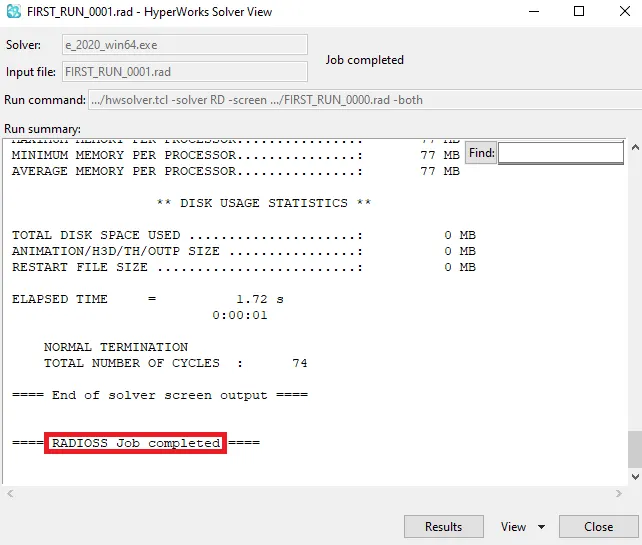
fig 4.9
Now, for checking whether the engine file is edited or not. Go to the file location, And open the file named "FIRST_RUN_0001.rad". Which shows the edited engine file, as shown in fig 4.10.
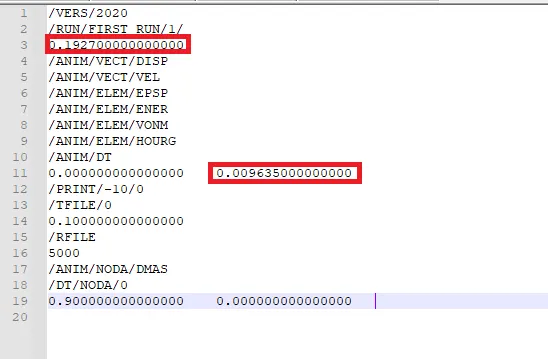
fig 4.10
5. To find: T frequency with respect to 20 animation steps:-
Formula used: Tfreq = Time step`-:`Number of animation steps
= 0.1927`-:`20
= 0.009635
Therefore, this T frequency value is entered in the card named " ENG_ANIM_DT", indicating that to produce 20 animation files. These files can be seen in the file location as shown in fig 5.1.
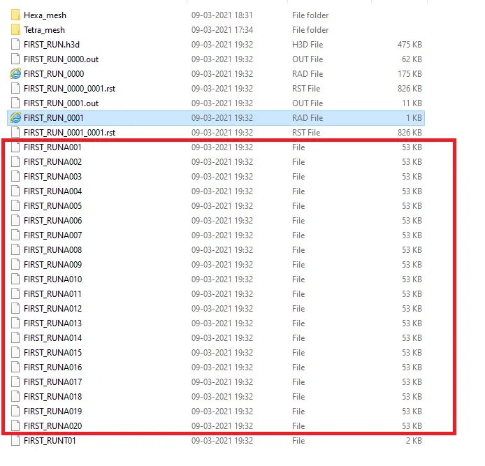
fig 5.1
6. To change the cycle with the spcific intervals difference of 10. This can be viewed, when the engine output file named"FIRST_RUN_0001.out" is opened. Which shows the entire cycle in number of dicrete cycles with the difference of 10, as shown in fig 6.1.
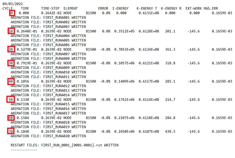
fig 6.1
7. Objective:
- To generate a 3D mesh (using tetra and hexa elements) on the given models. By following the given quality criteria.
Software used: Altair Hyperworks Desktop 2020
Procedure:
7.1 Model 1(Tetra meshing):-
Initially, the given model is imported in hyperwoks. After importing, the given model appears in the graphical display as shown in fig 7.1.1
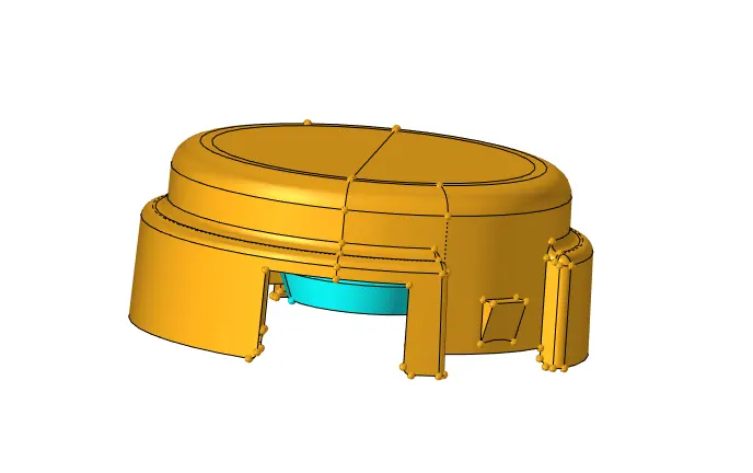
fig 7.1.1
The given model consists of two components (Cover and Hub). The cover component appears as shown in fig 7.1.2
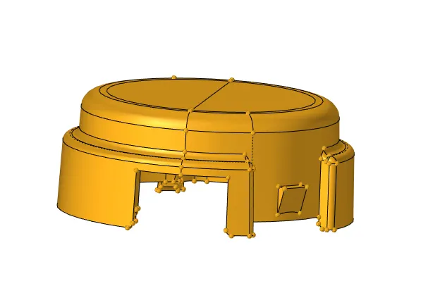
fig 7.1.2
The hub component appears as shown in fig 7.1.3.
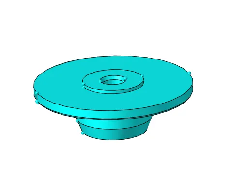
fig 7.1.3
The next step is to view the components by topo, In order to get a clarity on whether the given components comprises of solids or surfaces. And to view any geometry clean up is required. The cover component comprises of surfaces(Identified by clour: Grey colour represents the surfaces, Green colour represents the solids) as shown in fig 7.1.4.
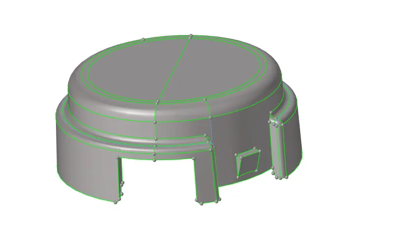
fig 7.1.4
The hub component also comprises of surfaces. It is viewed by topo as shown in fig 7.1.5.
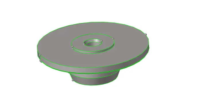
fig 7.1.5
Generating mesh:
The next step is to generate the mesh, Tetra meshing is done for this model. Before meshing, the quality criteria shold be set. The process for assigning this quality criteria is: Preferences(From Tool bar)---> Criteria file settings---> 3D---> assign the values---> Apply---> Ok. The criteria editor with the given quality criteria values entered is shown in fig 7.1.6.
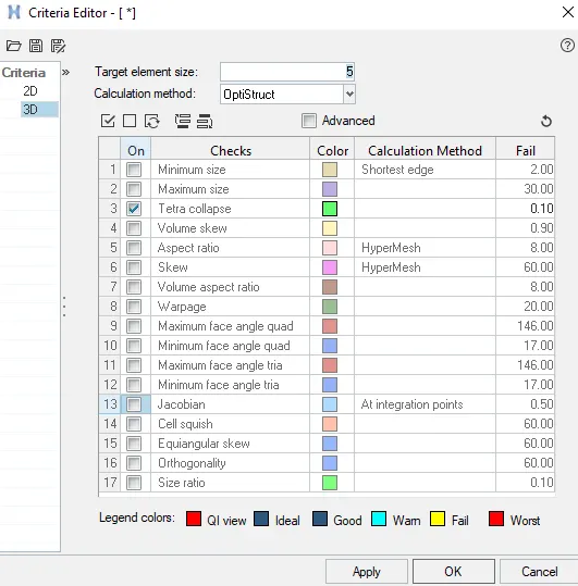
fig 7.1.6
The tetra meshing is done for the cover component by "Volume Tetramesh" option from the tetramesh in 3D panel as shown in fig 7.1.7. In general, the volume tetra mesh is done for the components with solids. But the volume tetra mesh can also be done for surfaces.

fig 7.1.7
After entering in to the volume tetra mesh panel, the surfaces to be meshed are selected & the given target element size "5 mm" is entered as shown in fig 7.1.8. Then by clicking on mesh, the mesh will be created.

fig 7.1.8
The meshed cover component appears as shown in fig 7.1.9.
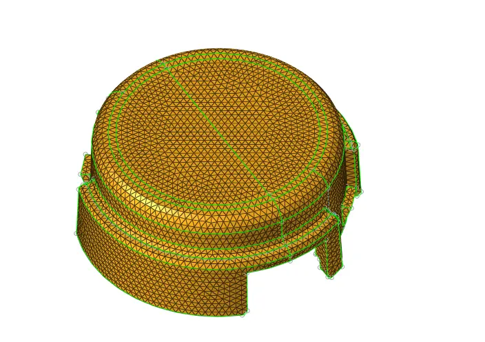
fig 7.1.9
Now, to know whether the component is meshed with tetra elements or not. Some of the elements are masked (Keyboard short-cut for mask is F5). After masking some elements, the component with tetra mesh appears as shown in fig 7.1.10.
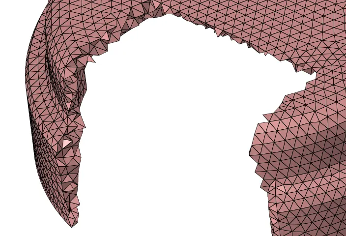
fig 7.1.10
The next step is to check for the quality criteria (i.e., Tet collapse). For checking the elements the keyboard short cut is F10(For check elements). which is shown in fig 7.1.11.

fig 7.1.11
The next step is to click on the "Tet collapse" , it will show the number of elements failing for tet collapse. As shown in fig 7.1.12, 113 elements are failing for tet collapse.
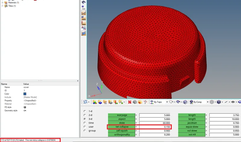
fig 7.1.12
The elements which are failing can be viewd by masking the remaining elements. This is done by the process: click on Save failed from F10---> Return---> click on F5---> elements---> Retrieve---> mask---> reverse all---> Failed elements will visible. The elements failing for tet collapse are shown in fig 7.1.13.
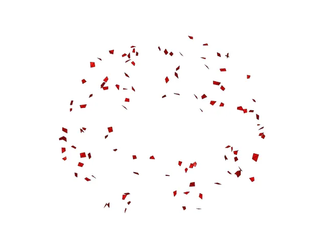
fig 7.1.13
This can be overcomed by tetra remesh from tetra mesh panel. This tetra remesh panel appears as shown in fig 7.1.14. In this panel, all elements should be selected and by clicking on remesh, the elements failed will be reduced or there will be no elements failing. If the elements failing are increasing after tetra remesh, then it would be a problem causedby the tet collapse value in tetramesh parameters. In tetramesh parameters, enter the required tet collapse value and then remesh.

fig 7.1.14
After remeshing, again the elements are checked for tet collapse by F10. Now there are Zero elements failing for tet collapse, as shown in fig 7.1.15.
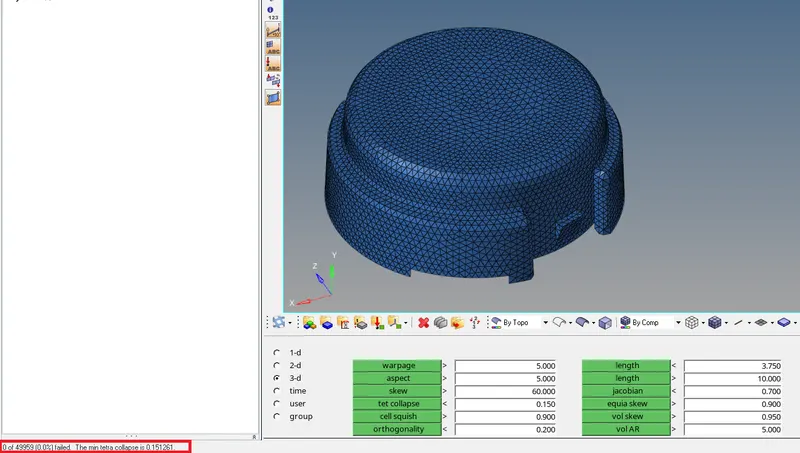
fig 7.1.15
For the next component(i.e., hub) the tetra meshing is done by using "Quick tetra meshing". The quick tetra mesh option is available in utility panel as shown in fig 7.1.16.
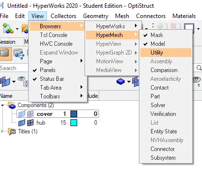
fig 7.1.16
After clicking on utility, the utility panel appears as shown in fig 7.1.17. In that the Option named "Geoemtry/mesh" should be selected.
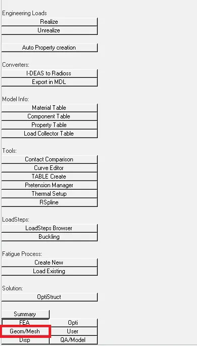
fig 7.1.17
Then the geometry/ mesh panel appears as shown in fig 7.1.18. In that the quick tetra mesh option should be selected.
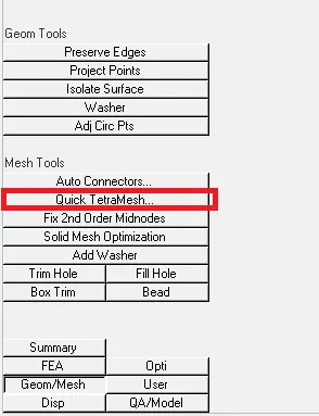
fig 7.1.18
Then the quick tetramesh panel appears as shown in fig 7.1.19. In that, some key parameters like components, mesh size( Target element length), mesh type should be selected. Then by clicking on mesh, the tetra mesh is created.
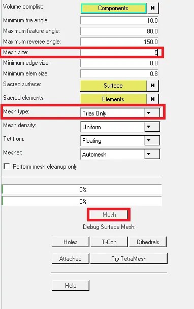
fig 7.1.19
The component is selected by double clicking on the components in quick tetramesh panel. Then a pop up comes at the bottom. There by selecting the components and by clicking on proceed, the component is selected as shown in fig 7.1.20.
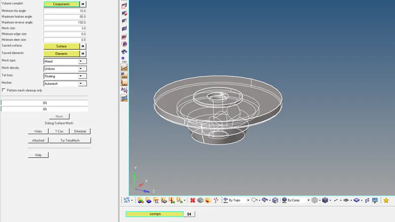
fig 7.1.20
After entering all parameters and clicking on mesh, It will take few moments. And then it generates a pop-up as shown in fig 7.1.21. Indicating that surface mesh is completed (i.e., 2D meshing) and attempted Tetra mesh(i.e., converted 2D to 3D automatically).
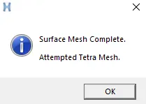
fig 7.1.21
After clicking "Ok", the component with the mesh appears as shown in fig 7.1.22.
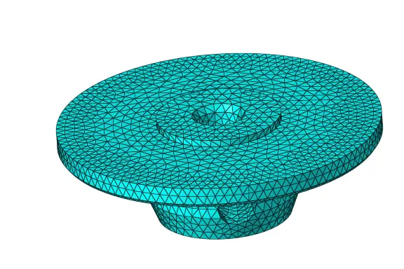
fig 7.1.22
Some elements are masked, In order to verify whether the component is meshed with tetra elements or not. After masking some elements, the component with tetra elements are shown in fie 7.1.23
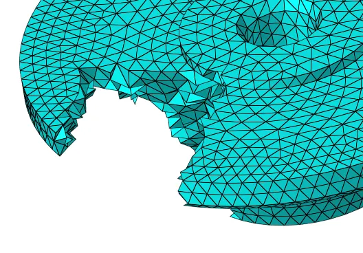
fig 7.1.23
The next step is to check the elements for tet collapse by F10. It is showing 61 elements are failing for tet collapse as shown in fig 7.1.24.
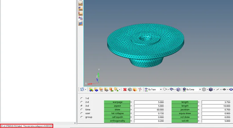
fig 7.1.24
The failed elements are shown in fig 7.1.25.
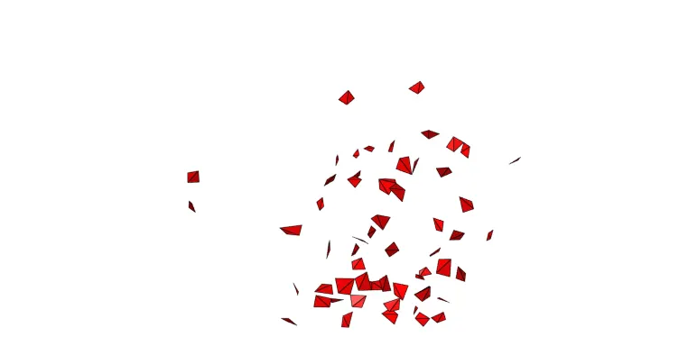
fig 7.1.25
Then the tetra remesh is performed. After remeshing, the elements failing for tet collapse is zero, as shown in fig 7.1.26.
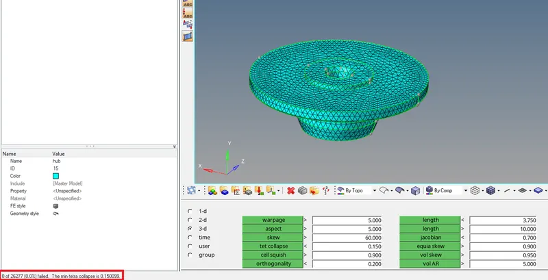
fig 7.1.26
Model 2(Hexa meshing):-
Initially, the given model(Arm bracket) is imported in hyperworks. After importing, the model apppears in the graphical display as shown in fig 7.2.1.
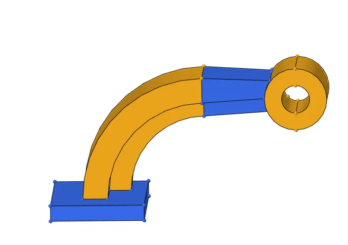
fig 7.2.1
The next step is to view the given model "By Topo". The given model by topo appears as shown in fig 7.2.2.
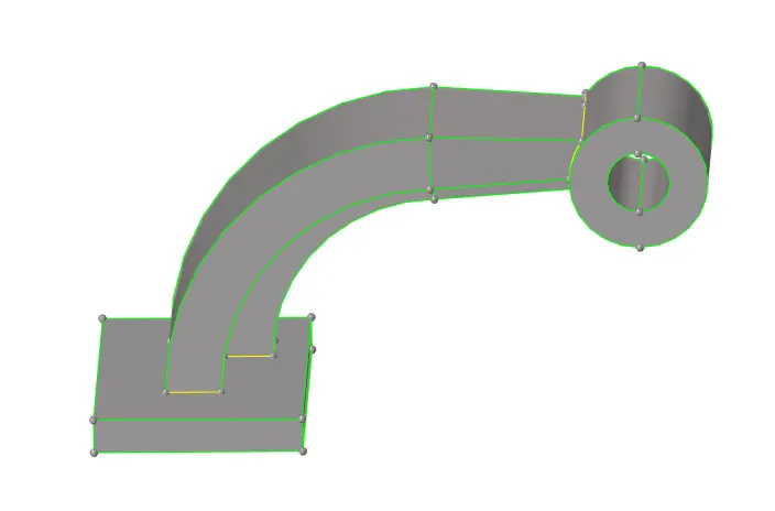
fig 7.2.2
The given model contains four components. They are: Base, arm curve, arm straight, boss. Initially, the meshing is done for base component. The base component appears as shown in fig 7.2.3.
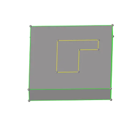
fig 7.2.3
Firstly, 2D meshing should be done on one surface with first order quad elements( quad element with 4 nodes), In order to create the 3D hexa elements. For that, as usually the automesh panel is opened from 2D and some psrameters such as element size, enabling the align, size of flow, selecting the surface as shown in fig 7.2.4. Inorder to have a proper mesh flow. And then click on mesh.

fig 7.2.4
After meshing with 2D quad elements, the mesh appears as shown in fig 7.2.5
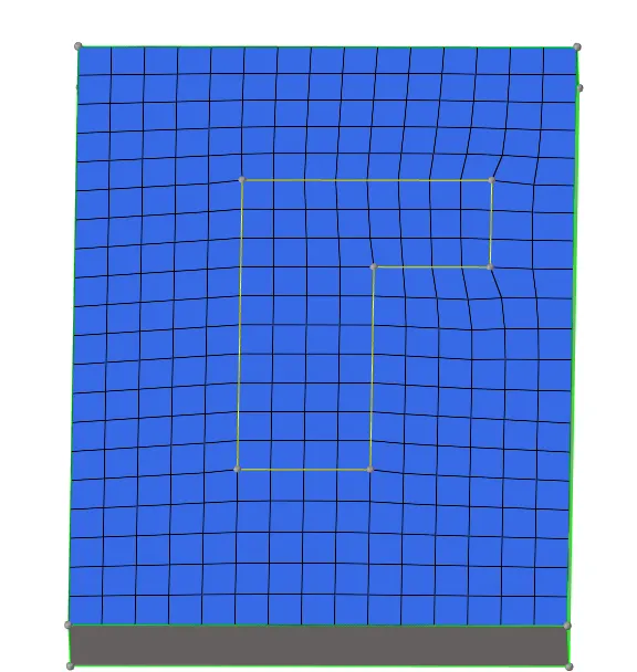
fig 7.2.5
The next step is to create the 3D elements with reference to this 2D elements. The option used for doing 3D meshing of base component is "Element offset". This option is available in 3D panel as shown in fig 7.2.6.

fig 7.2.6
After entering in to element offset, Some parameters such as, the 2D elements to be offset is selected, And surfaces are selected to mention alond the the geometry on which the elements to be offseted, Number of layers, Total thickness are assigned as shown in fig 7.2.7. Then by clicking on offset, the 3D hexa elements are created.
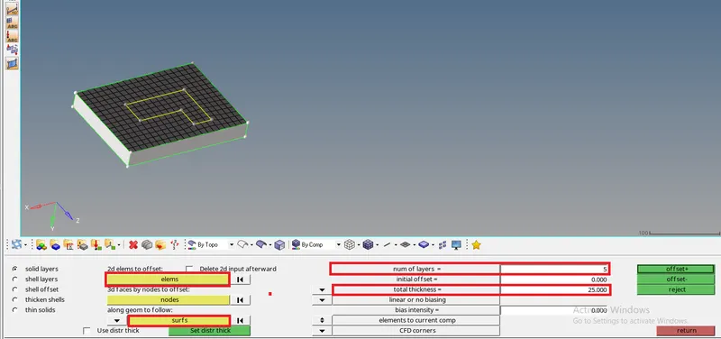
fig 7.2.7
The created hexa meshing for base component apppears as shown in fig 7.2.8.
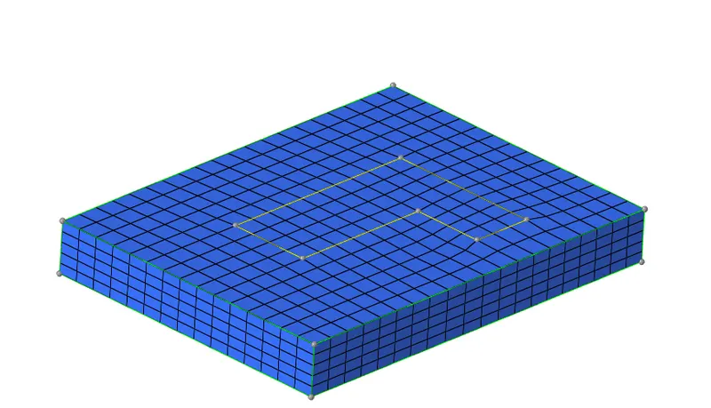
fig 7.2.8
Inorder to know whetther the hexa elements are created or not, some elements are masked. The base component with hexa elements is shown in fig 7.2.9.
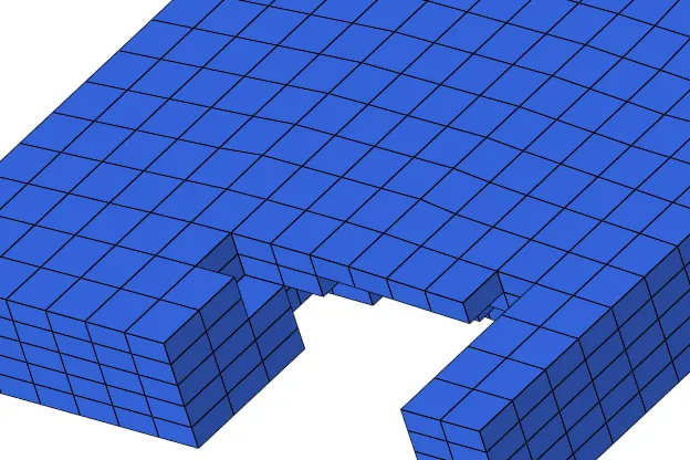
fig 7.2.9
Note: Eventhogh the hexa meshing is created, the 2D shell elements used for generating the 3D mesh will be there. These elements should be deleted at the end.
The next component is arm curve. This component is enabled and the created hexa mesh for base component is masked. Inorder to use the 2D quad elements for meshing the arm curve also as shown in fig 7.2.10.
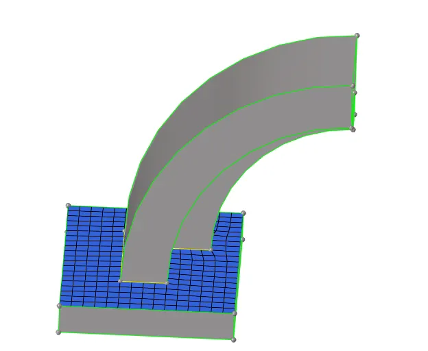
fig 7.2.10
The tool used for generating the hexa mesh for this component is "Spin" from 3D panel as shown in fig 7.2.11.

fig 7.2.11
Inorder to spin the elements , a center is required as a base node. For getting that node, the option used is "Distance" (Keyboard short-cut is F4). And by using three nodes (circle center) as shown in fig 7.2.12.
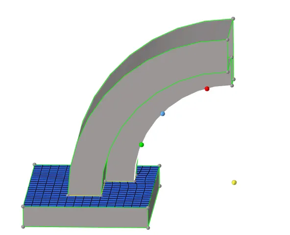
fig 7.2.12
Then by using the spin option, the elements to be spin, axis to which the elements should spin (X- axis), Base node, angle (90 degrees), number elements required on spin are selected as shown in fig 7.2.13 . And by clicking on spin, the 3D mesh is created
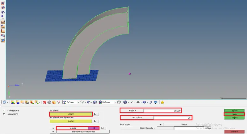
fig 7.2.13
The generated mesh on arm curve appears as shown in fig 7.2.14.
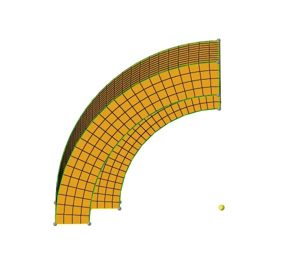
fig 7.2.14
To verify whether, the generated mesh is a 3D mesh or not, some elements are masked as shown in fig 7.2.15.
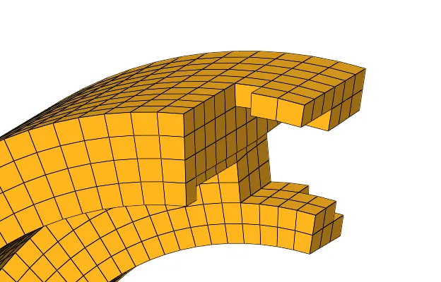
fig 7.2.15
The next component to be meshed is arm straight. It is enabled as shown in fig 7.2.16.
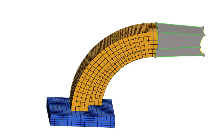
fig 7.2.16
For meshing this component, the tool used is "Linear solid". So, it should have the elements in both source geometry and destination geometry. For the source geoemtry to have 2D quad elements, the faces are finded. This is done by using "Faces" tool in tool panel from main menu bar. The component is selected and by clicking on "Find faces" as shown in fig 7.2.17, the faces are otained

fig 7.2.17
The obtained faces will be shown in different colour as shown in fig 7.2.18.
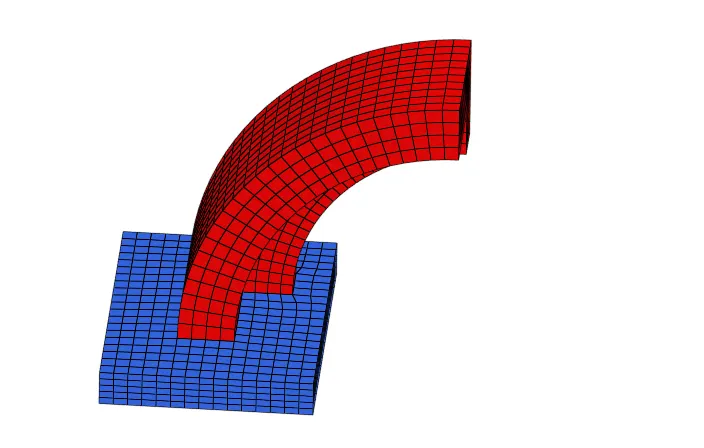
fig 7.2.18
Then the 2D mesh should be created, in the destination surface with the same number of elements as shown in fig 7.2.19.
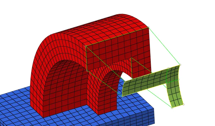
fig 7.2.19
The next step is to select the elements from source surface to destination surface and the planes are also selected in the same way and the density of the mesh( Number of elements in between tose surface) are selected as shown in fig 7.2.20. By clicking on solids, the 3D mesh is created.
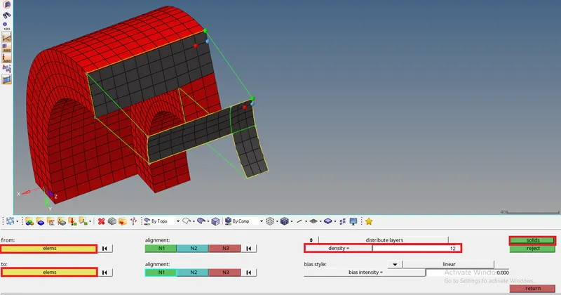
fig 7.2.20
The generated mesh appears as shown in fig 7.2.21.
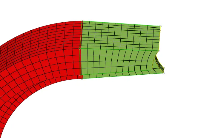
fig 7.2.21
In order to verify whether the generated mesh comprises of hexa elements, some elements are masked, as shown in fig 7.2.22
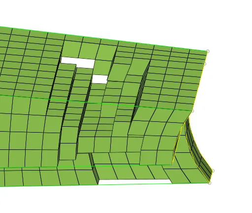
fig 7.2.22
The next component to mesh is the boss. The option used for generating the mesh for this component is "Solid map". This component is enabled, as shown in fig 7.2.23.
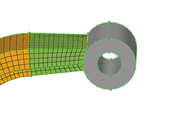
fig 7.2.23
Initially, one side surface is meshed with 2D quad elements as shown in fig 7.2.24.
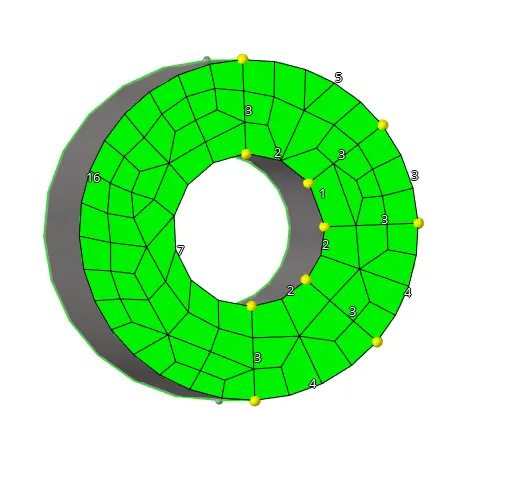
fig 7.2.24
The same number of nodes should be there at both ends as shown in fig 7.2.25. Inorder to have the quad elements.
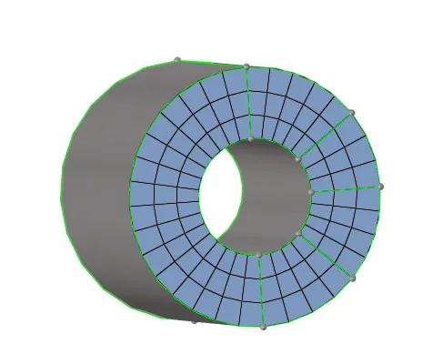
fig 7.2.25
The next step is to create a node at the destination surface by duplicating the node at the end of the mesh as shown in fig 7.2.26. This duplicated node is projected to the surface. ( Keyboard short-cut for project is Shift+F7).
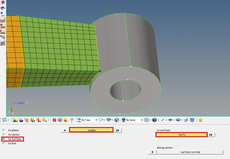
fig 7.2.26
After projecting the node to destination surface, it appears as shown in fig 7.2.27. This node is projected to have proper mesh flow and the alignment after creating the mesh on the boss component.
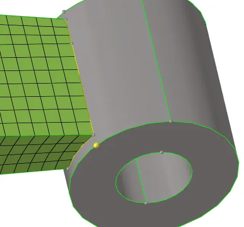
fig 7.2.27
Now With the help of a solid map tool, the destination surface, the elements to be mapped, nodes to which the connectivity should be there are selected as shown in fig 7.2.28. For better understanding to the solver, lines along which the mesh should be generated are also selected.
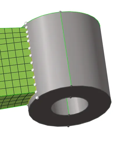
fig 7.2.28
After generating the hexa mesh, it appears as shown in fig 7.2.29. The next step is to check for the connectivity for the elements in the arm straight component and boss component. If there is no connectivity, use the replace node option(F3) or equivalence(Shift+F3).
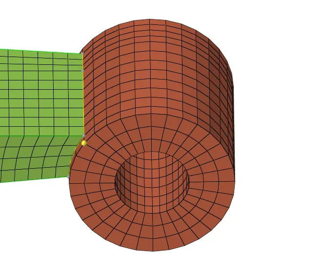
fig 7.2.29
To know whether the formed elements are hexa or not, some elements are masked as shown in fig 7.2.30.
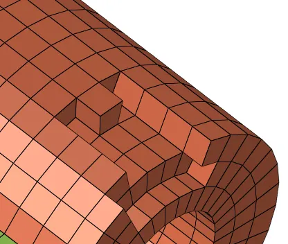
fig 7.2.30
The final model with the entire hexa meshed appears as shown in fig 7.2.31.
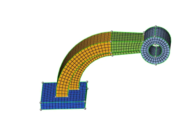
fig 7.2.31
Conclusion:
- Generated a 3D mesh (using tetra and hexa elements) on the given models. By following the given quality criteria.
Learning outcomes:
By doing this challenge, the following concepts can be understood:-
- Some calculations such as speed of sound, time step, T frequency values.
- Types of files in radioss like starter & Engine files.
- Editing of engine file.
- 3D meshing using tetra & Hexa elements.