Assignment 7-Side Pole Crash Simulation Challenge

1. Objective:

• To bring the center of gravity near to the driver seat.
• To create the sections on cross members.
• To create intrusions.
• To give the initial velocity.
• To give the connections(If necesscary).
• To create the interfaces.
• To request for the outputs, by assigning the TH.
• To plot the results by using various graphs.

2. Software used: Altair Hyperworks Desktop 2020

3. User Profile: Radioss

4. Abstract:

Statistics:- For fatalities, in the United States, in 2008, a total of 5,265 (22%) out of 23,888 people were killed in vehicles which were struck in the side. For speed, in Europe in 2015, it is considered that best designed cars provide serious front crash protection with speeds up to 70 km/h for car occupants wearing seat belts in frontal impacts and 50 km/h in side impacts. It is considered that passenger car fatalities and seriously injured side impacts account for about 35 to 40%. In European countries, such as UK, Sweden and France, around one quarter of traffic injuries are produced by side collision, but among people subject to killing injuries the side impact account for 29 to 38% of those fatal injuries. So, the side crash test is mainly done in middle eatern countries.

                  To overcome the problems with respect to the side crash, an explicit analysis is done using radioss. And the post-processing is done using hypermesh & hypercrash. In this analysis, a pole with the diameter of  254 mm(recommended as per the FMVSS standards) is used as a rigid body. And the crash is done with the angle of 90 degrees with the velocity of 35 miles per hour. And the obtained errors are viewed by graphs in the post-processing phase.

5. Procedure:

Step 1: Bringing the center of gravity near to the driver seat:-

This step is done in Hypercrash. Because, In hypercrash we can set up the deck.

To open the hypercrash, the hypermesh is opened. And in that, by clicking on applicatins tab in the menu bar. The hypercrash option is available as shown in fig 5.1.

                                               

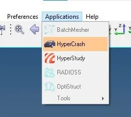
                                                                          fig 5.1

After a while, a dialog box appears as shown in fig 5.2. In order to set up the unit system. The preffered unit systems are (Mg, mm, s) or (Kg, mm, ms). Because they were used widely in the industries.

                                      

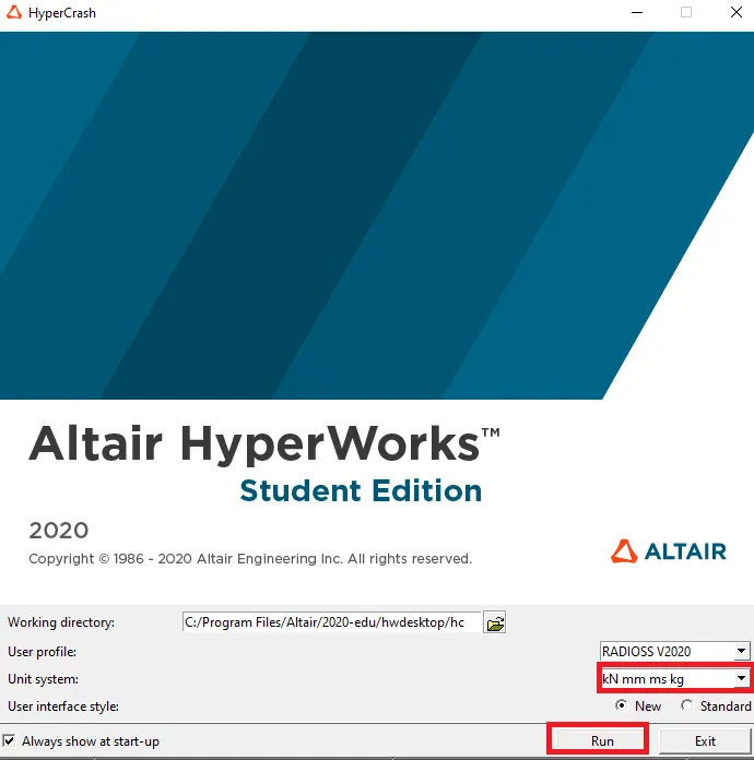
                                                                        fig 5.2

After selecting the unit system, by selecting the "Run" the hypercrash user interface appears as shown in fig 5.3. Meanwhile, it takes few moments to open. 

                       

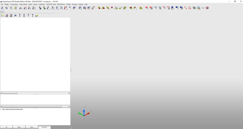
                                                                               fig 5.3

Then the starter rad file is imported. After importing, the given meshed model appears in the graphical area of hypercrash interface as shown in fig 5.4.

                                   

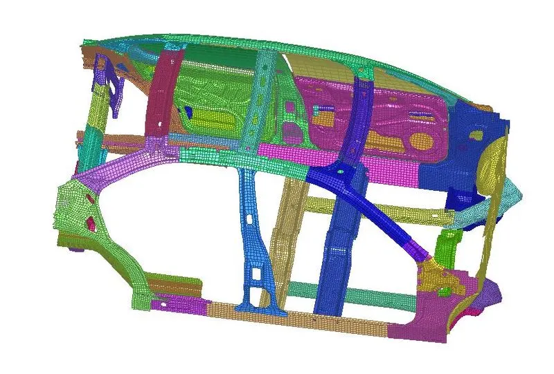
                                                                                          fig 5.4

Then next step is to check for the center of gravity of the given model. In order to view that, the option named "Mass" in the menu bar is choosed. In that "Balancing" option is selected, as shown in fig 5.5. 

                                                              

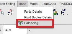
                                                                                       fig 5.5

In that, an option which is highlighted in the fig 5.6 is selected to view the initial center of gravity. And it also shows the mass present on the model (166 kg as shown in fig 5.6). This should be increased to 700 kg, as mentioned in the question. Inorder to get the center of gravity at the required position.    

                                     

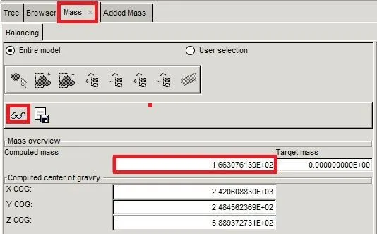
                                                                         fig 5.6

After choosing that option, the center of gravity is shown in the form of a small point as shown in fig 5.7.

                                      

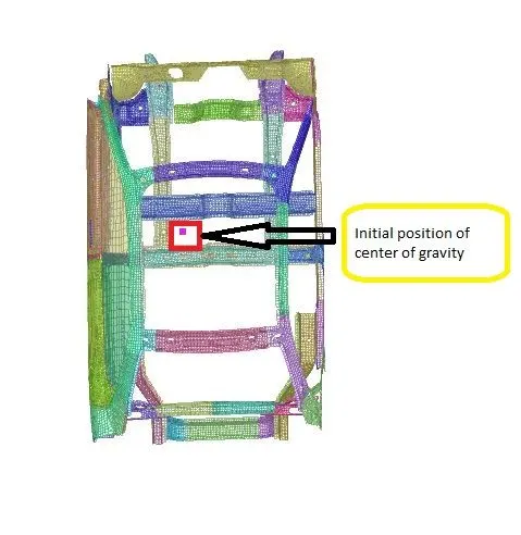
                                                                               fig 5.7

Inorder to bring that to our required position, the masses should be added to the nodes. For adding the masses, "Addded mass" option in the loadcase is choosed as shown in fig 5.8.

                                      

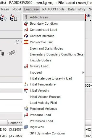
                                                                             fig 5.8

After selecting that, by right clicking on the tab bar. A pop-up appears as shown in fig 5.9. To create new masses. In that, the type 1 is selected. Inorder to disribute the given mass to each node of the node group selected. 

                                      

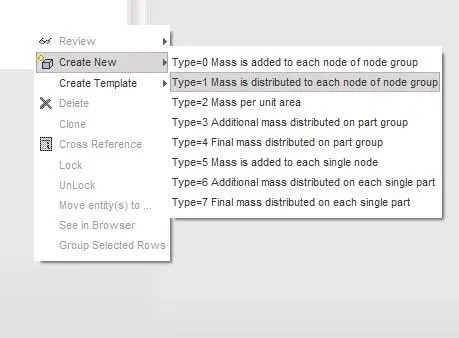
                                                                                fig 5.9

After selecting that, a new compoent in the tab bar appears as shown in fig 5.10. To assign the parameters such as mass(in Kg), grnod_ID( group of nodes to which the mass should be distributed). After selecting the group of nodes, an option "Yes" will be there at the bottom, to confirm the nodes. This nodes selection is done by righ clicking on the nodes option, as shown in fig 5.10.

                                      

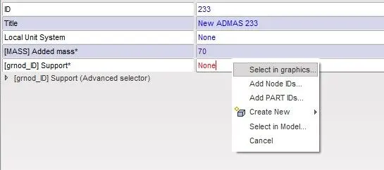
                                                                                   fig 5.10

By clicking that, a pop-up appears as shown in fig 5.11. In that, the first option is selected, to select the nodes.

                                      

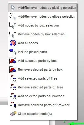
                                                                            fig 5.11

The nodes are selected and assigned the masses, the assigned masses are shown in the form of names as shownin fig 5.12. 

                                      

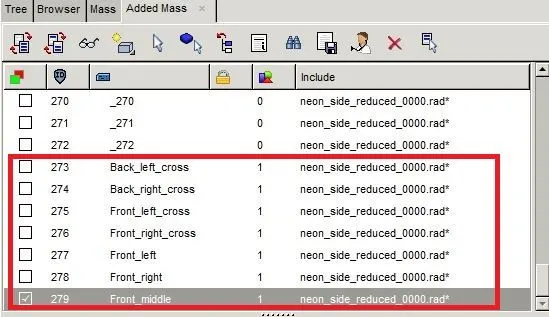
                                                                              fig 5.12

The selected nodes with assigned masses are highlighted, as shown in fig 5.13.

                                      

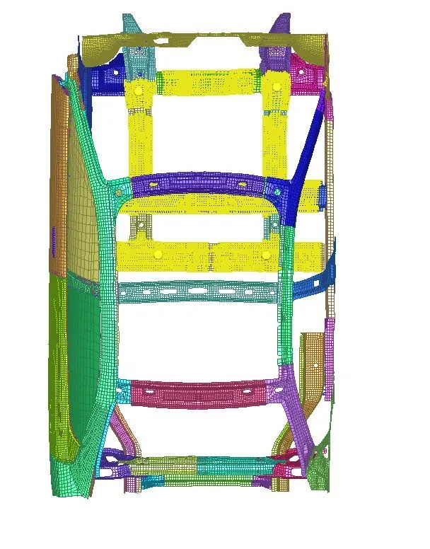
                                                                                 fig 5.13

After adding those masses till 700 kg, the change in center of gravity is shown in fig 5.14. Which is the required position.

                                     

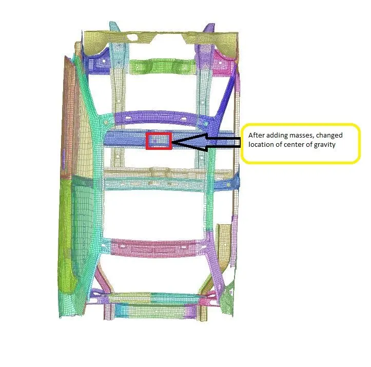
                                                                          fig 5.14

Step 2: Creating sections:-

The model with the obtained COG is exported to some file location. ANd this file is imported in hypermesh. After importing the solverdeck in hypermesh, the model in the graphical display appears as shown in fig 5.15.

                                        

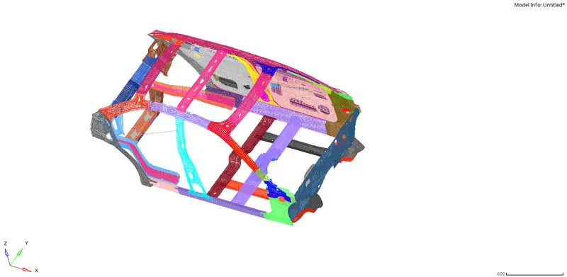
                                                                             fig 5.15

Inorder to view whether the imported model consists of same mass or not, the mass, COG option is used.The process of selecting that option is: Tools in menu bar---> Mass details---> Mass,COG & Inertia. After selecting that option, a pop-up appears as shown in fig 5.16. Indicating the mass details.

                            

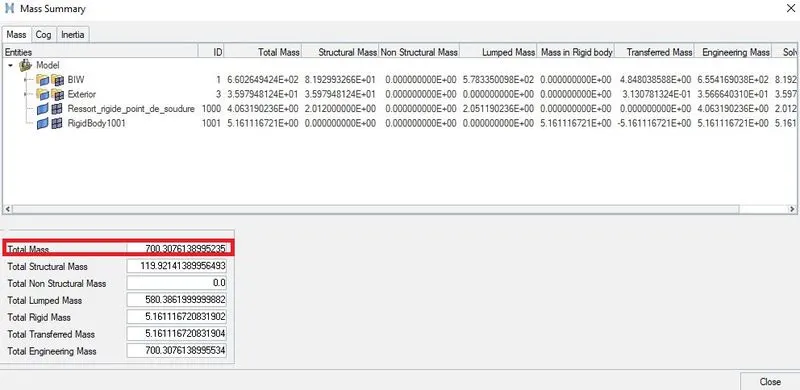
                                                                                       fig 5.16

 For creating the sections, frames are needed first. So for craeting a frame, three nodes are required. To specify the origin, Z-axis, YZ-plane as shown in fig 5.17. The process of creating a frame is: Right click on the tab bar in solver browser---> Create---> Frame---> Selecting the three nodes.

                            

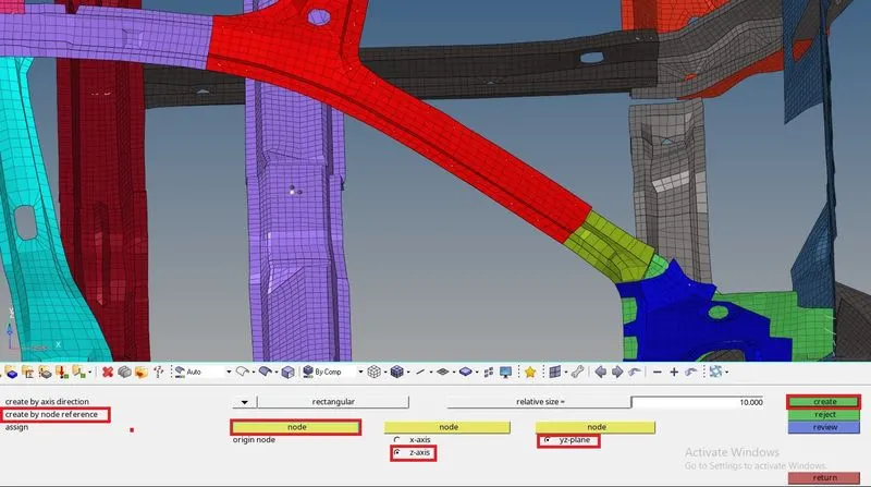
                                                                                                fig 5.17

After creating the frame, the obtained frame appears in that location as shown in fig 5.18.

                                                                    

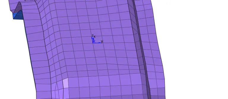
                                                                                                       fig 5.18

The next step is to create the section. The process of creating the section is:  Right click on the tab bar in solver browser---> Create---> SECT--> SECT_CIRCLE---> Assigning the frame in the parameter window---> Select some elements. After creating the section, it appears as shown in fig 5.19.

                                                                    

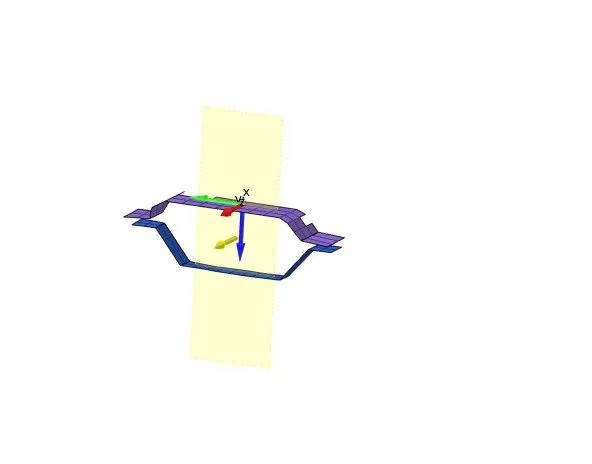
                                                                                                 fig 5.19

As mentioned in the question, the sections should be created on two cross members,  to know how much force is travelling through that member. After creating the sections on that members, it appears as shown in fig 5.20

                                                               

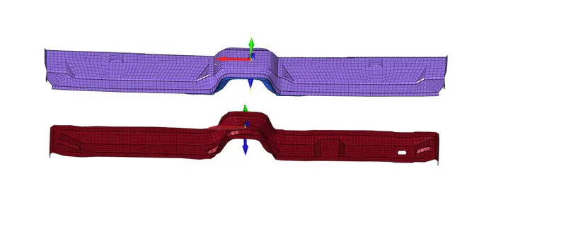
                                                                                                   fig 5.20

Step 3: Creating intrusions(Springs):-

The next step is to create the springs, To know the intrusions(Deflection). So for creating that, the process is: Open 1D panel from main menu page---> Springs---> Select (Spring2) Spring with 2 nodes, as shown in fig 5.21.                                                            

                                                          

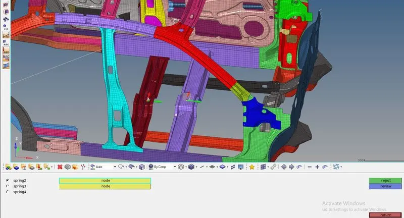
                                                                                       fig 5.21

In the same way, three springs are created near fuel tank region, B pillar, Hinge pillar regions. As shown in fig 5.22.

                                                          

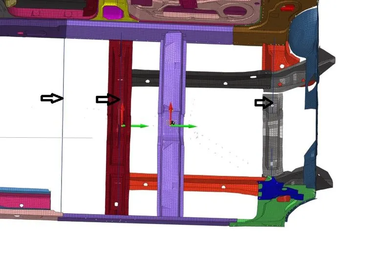
                                                                                          fig 5.22

The next step is to assign the mass and stiffness values for the created springs, in the parmeter region, as shown in fig 5.23.

                                                          

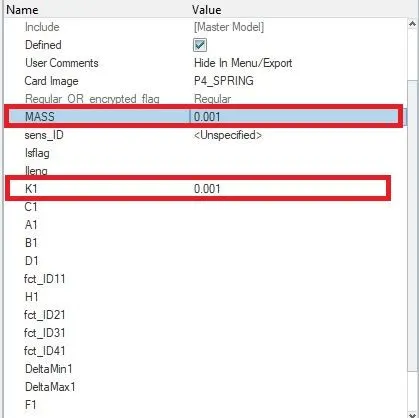
                                                                                             fig 5.23

The next step is to create the properties for springs. And assigning the created property to the spring, as shown in fig 5.24. 

                                                           

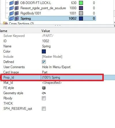
                                                                                               fig 5.24

Step 4: To obtain the peak velocity at the given node(337773):-

In this step, the node with the value 337773 should be founded. The process of finding that node is: Select the option "Display numbers" as shown in fig 5.25---> Right click on "nodes" option---> click on "By Id"---> Click "ON".

                                                                                        

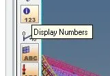
                                                                                                    fig 5.25

After displaying that node, it appears as shown in fig 5.26.

                                                             

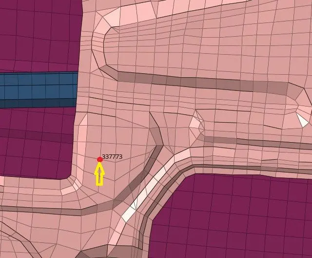
                                                                                                      fig 5.26

The next step is to create a TH for that node. Because, to know the peak velocity at that point. So, it is requested with the help of TH. The process of creating the TH for that node is:  Right click on the tab bar in solver browser---> Create---> TH---> NODE. The created TH in the tab bar appears as shown in fig 5.27.

                                                                             

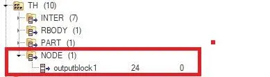
                                                                                                         fig 5.27

Then in the parameters window, the node should be given with the translation velocity in X,Y,Z direction, as shown in fig 5.28.

                                                             

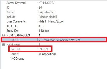
                                                                                                          fig 5.28

Step 5: Creating a rigid wall:-

The next step is to give the connections between the components, as shown in fig 5.29. If there is no connections between the components, then   the force is not transfered to the other components. Which leads to the components fly when the load is applied. 

Note: The connections should be checked thoroughly, Before running the simulation.

                                                             

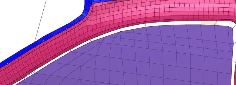
                                                                                                      fig 5.29

Then three nodes should be created (Two nodes in Y-axis & one node in X-axis. The distance between the nodes depends on user), as shown in fig 5.30. These nodes will help to form the rigid wall.

                                                             

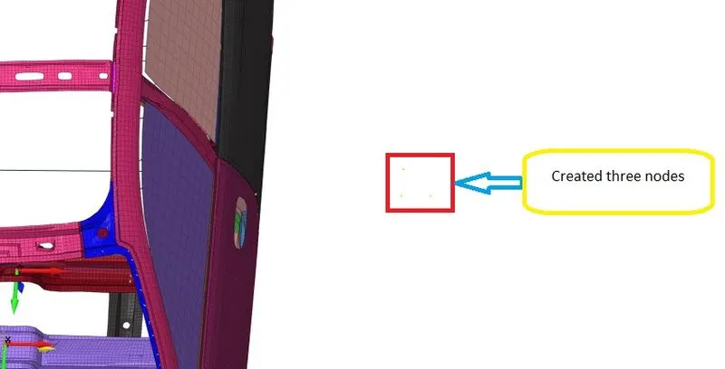
                                                                                              fig 5.30

In the paramater window, the (XM,YM,ZM) should be selected. It is selcted by, cliking on the origin node. And the Normal is selected, by selecting the created three nodes as shown in fig 5.31. And the few parameters such as Friction, diameter of the cylindrical pole (Rigid), Searching tolerance(Dsearch).

Note: The diameter of the created pole is taken as 254 mm(Recommended value as per FMVSS standards).

                                                             

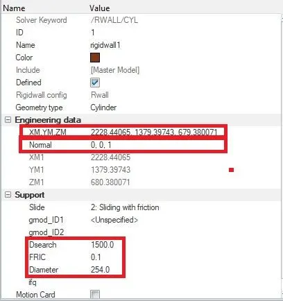
                                                                                             fig 5.31

After entering those values, the created rigid wall appears as shown in fig 5.32.

                                                             

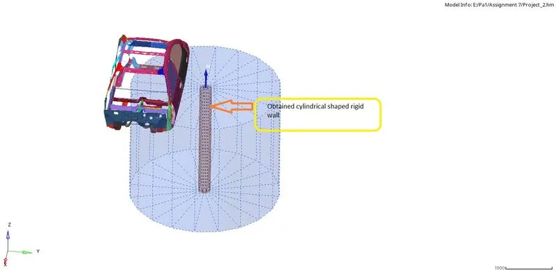
                                                                                                  fig 5.32

Step 5: Creating new interfaces:-

Initallly, By default the model will have some interfaces pre-defined. As shownin fig 5.33.

                                                           

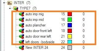
                                                                                          fig 5.33

So, the new interfaces are created. The process of creating the interface is: Right click on the tab bar in solver browser---> Create---> INTER---> Select the type of contact required(eg: Type 7). After creating the interface, the parameters for that are to be entered,as shown in fig 5.34.

                                                          

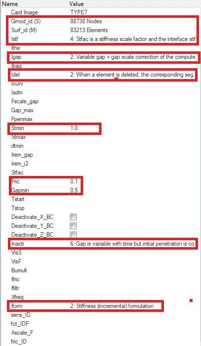
                                                                                                fig 5.34

Step 6: Assigning the initial velocity:-

The next step is to assign the initial velocity. The process of creating the initial velocity is: Right click on the tab bar in solver browser---> Create---> BOUNDARY CONDITIONS---> INIVEL.  After creating that in the parameter window, the velocity components should be mentioned as shown in fig 5.35. And the initial velocity given is 15.646 m/s in Y-axis(Because, the car need tohit the rigid wall in Y-axis).

                                                          

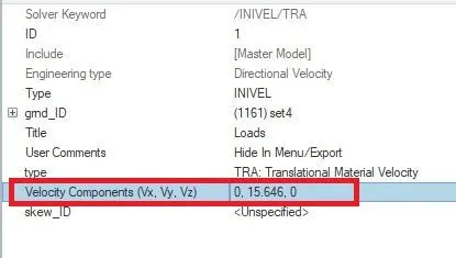
                                                                                               fig 5.35

The next step is to request the outputs for the assets, as shown in fig 5.36

                                                          

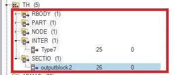
                                                                                                   fig 5.36

Then the post processing is said to be almost completed. The final step is to run the model checker. The process for getting the model checker browser  is: Tools in menu bar---> Model checker---> In the tab bar right click & select the option "Run". After a while, it shows the errors, warnings & INFO. After completing, if there is no errors as shown in fig 5.37 then the simulation can be runned. 

                                                          

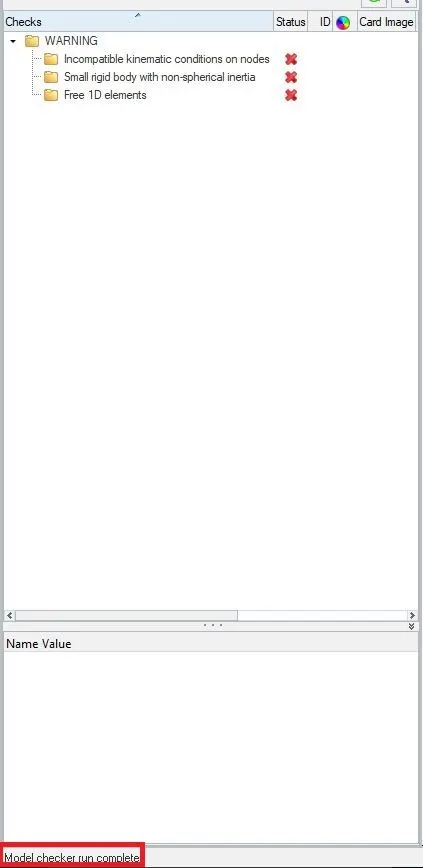
                                                                                                   fig 5.37

Step 7: Running the simulation:-

The simulation is runned by using the radioss option in the analysis panel, as shown in fig 5.38. Before running the simulation, the file should be saved in some location. In order to store the obtained animation files.

                      

                                                                                                      fig 5.38

After running the simulation, the obtained files in the specified location appears as shown in fig 5.39.

                                                          

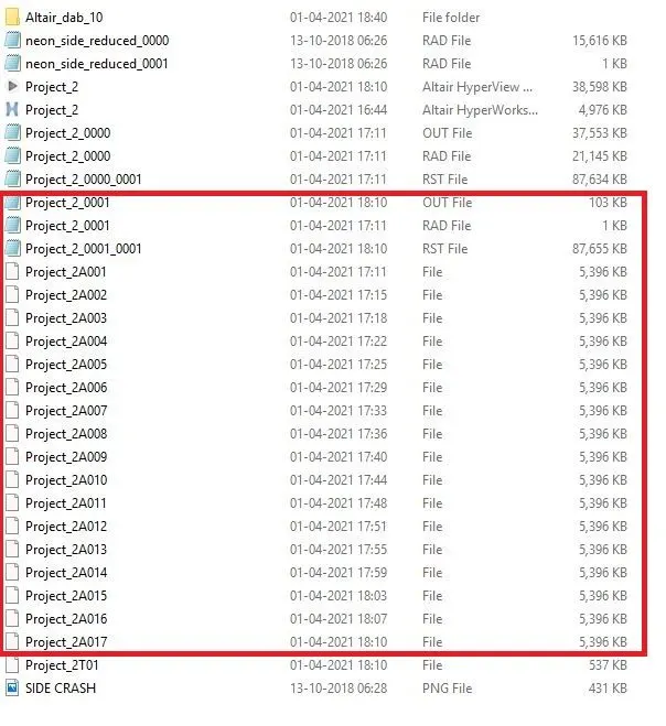
                                                                                                  fig 5.39

After running the simulation, a pop-up appears, indicating "Radioss job completed". Then from the obtained 0001.out file, the results in the form of values are seen. The obtained values for the last cycle is shownin fig 5.40.

                                                           

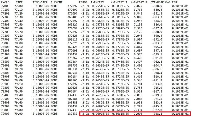
                                                                                                fig 5.40

Then the h3d file is imported in the another window, Inorder to view the simulation. After importing the h3d file, the graphical display appears with the model & rigid wall as shown in fig 5.41. 

                                                 

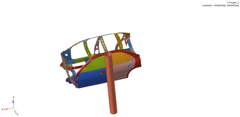
                                                                                                         fig 5.41

Then in the hyperview the contour option is selected. In order to selct the parameters such as the result type, selection of components etc. The contour panel appears as shown in fig 5.42. After clicking on "Apply", the result can be viewed.

                                                                                                   fig 5.42    

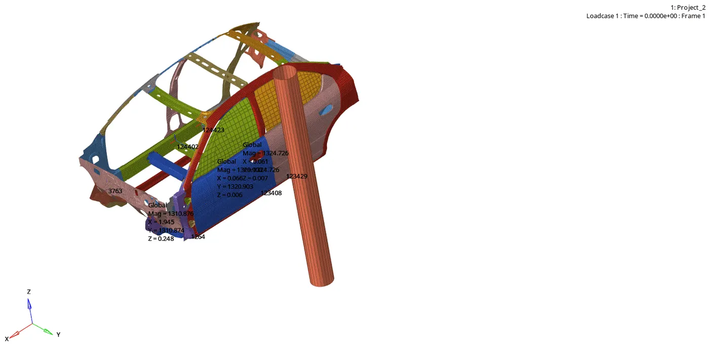
The obtained simulation in the mesh view appears as shown in the below animation.

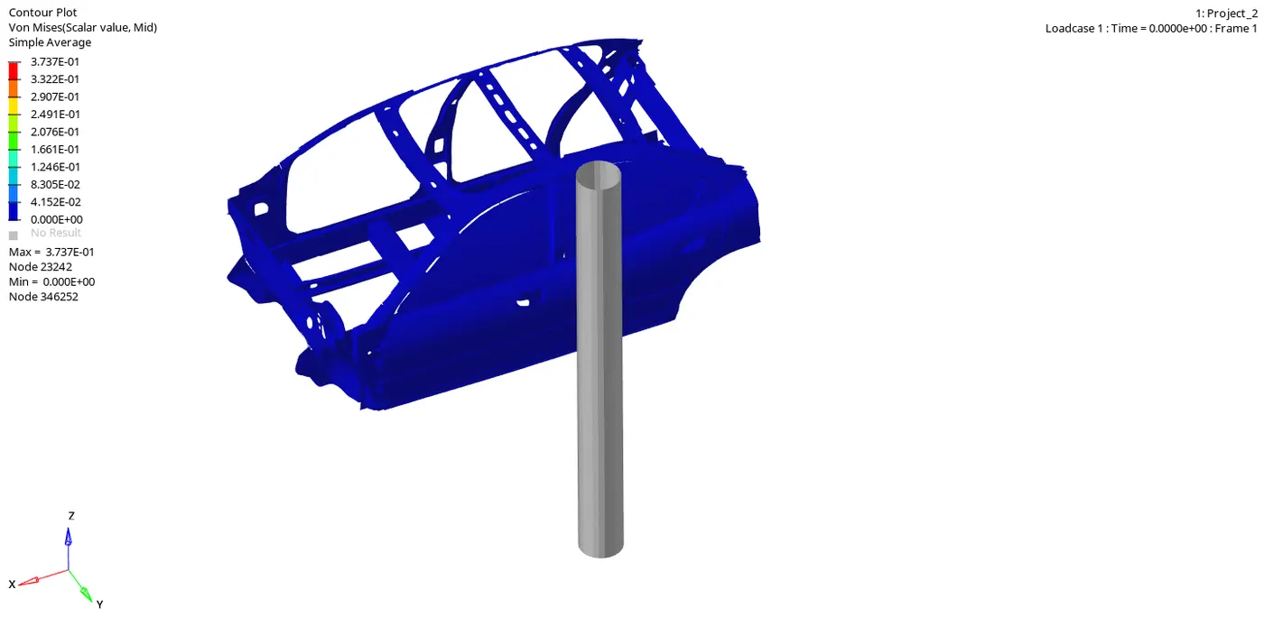
The obtained simulation interms of von-mises appears as shown in the below animation.

Step 8: Post processing:-

Post-processing is the final step. Where the obtained results are seen in the form of graphs.  This is done by importing the T01 (Time history) file in other window(With in Hypergraph 2D panel), as shown in fig 5.43.

   

                                                                               fig 5.43

After importing that, the unit system selection is done before applying the required result as shown in fig 5.44. In that the units to be selected are shown in column D.

                                    

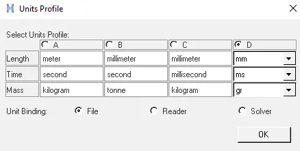
                                                                                   fig 5.44

The parameters to be selected for obtaining the sectional forces in the cross members are shown in fig 5.45.

The next step is to obtain the graphs with respect to that unit system. Firstly, the graph obtained is the sectional force in both the cross members. Which appears as shown in fig 5.46. From that fig we can notice that, the sectional force experienced by the first cross member is more than the second cross member.

  

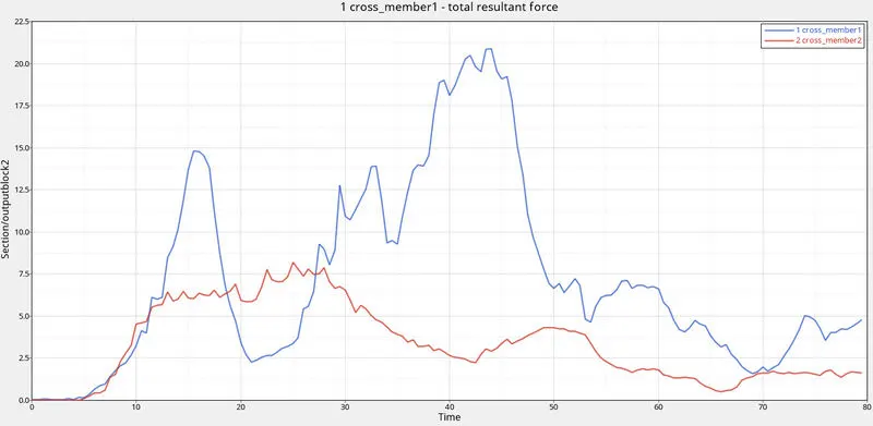
                                                                                fig 5.46

Then a graph is plotted in terms of interfaces. The parameters to be selected for obtaining the force by the interfaces are shown in fig 5.47. 

                                                                                  fig 5.47

The obtained total resultant force for the interfaces is shown in fig 5.48. The interface foces reaches to a peak value, when ther is a collision. And it gradually increases & decreases before it reaches to peak value is because, there will be a contact forces acting with in the car before collision.

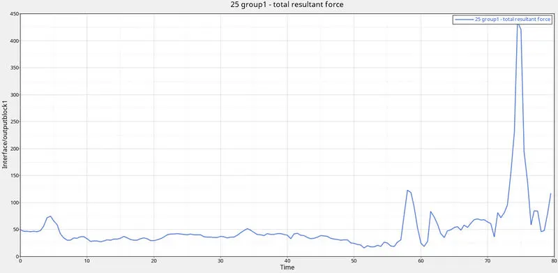
                                                                           fig 5.48

The next step is to find the intrusion happened by the means of springs. For that, the distance option is used in the hyperview panel, as shown in fig 5.49.

                                                                               fig 5.49

After clicking on that distance option the springs are selected. This process of selecteing the springs is done twice. One is at the initial stage. Showing the magnitude as 1310.876mm for the first spring (At hinge pillar), 1324.725mm for the middle spring(At B-pillar) & 1320.903mm for the last spring(At fuel tank), as shown in fig 5.50.

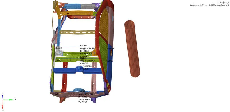
                                                                    fig 5.50

Then for the next time, after deflection the distance is measured. But this time, the obtained magnitude for first spring is 1237.481mm, middle spring is 730.955mm & for the last spring the obtained magnitude is 690.075mm, as shown in fig 5.51.

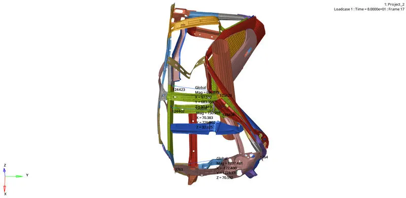
                                                                                      fig 5.51

The difference between the obtained magnitudes, will give the intrusions at that regions.

For first spring:(At hinge pillar)---> Intrusion = 1310.876 - 1237.481 = 73.395 mm

For second spring:(At B-pillar)---> Intrusion = 1324.725 -  730.955 = 593.77 mm

For third spring:(At fuel tank)---> Intrusion = 1320.903 - 730.955 = 589.948 mm

From the above results, the intrusion in the springs with descending order is B-pillar, Fuel tank, Hinge pillar.

Then the graphs for this intrusions can be obtained in two ways:

1. First one is from the selection of nodes of the springs at the beginning. By selecting the option named " Create curve",as shown in fig 5.52.

                                                                              fig 5.52

     2. The second way is directly going to the hypergraph 2D panel and selecting the parameters, as shown in fig 5.53.

                                                                                fig 5.53

The obtained graph for the total length resultant elongation for first spring is shown in fig 5.54.

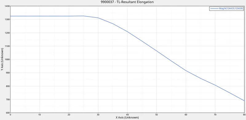
                                                                     fig 5.54

The obtained graph for the total length resultant elongation for second spring is shown in fig 5.55.

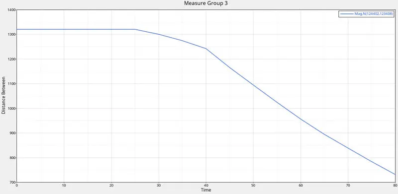
                                                                            fig 5.55

The obtained graph for the total length resultant elongation for third spring is shown in fig 5.56.

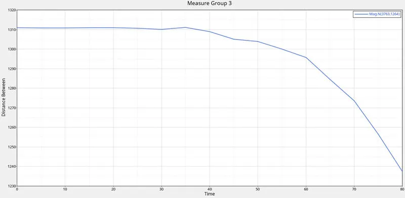
                                                                              fig 5.56

The intrusion in all three springs are shown in fig 5.57.

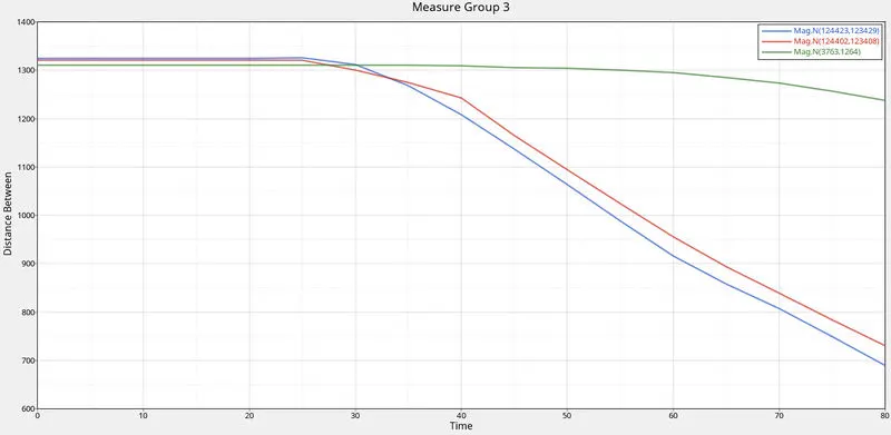
                                                                                 fig 5.57

The next graph obtained is for knowing the peak velocity at the node 337773. The parameters are selected to obtain the graph are shown in fig 5.58.

                                                                                  fig 5.58

The obtained peak velocity at the node 337773 is 16.0014m/s, as shown in fig 5.59. The reason for the velocity not starting from the origin is, Inertia. At the beginning of collision the car starts moving towards rigid wall And not attains to the rest condition all of a sudden. Due to inertia.

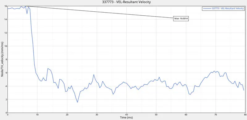
                                                                                   fig 5.59

The final graph obtained is in trems of energies, as shown in fig 5.60. The reason for the behavior of those energies are listed below:

• Kinetic energy: The kinetic energy will decrease due to the decrease in velocity after collison. So, it gradually decreases with respect to time.
• Internal energy: The fall in kinetic energy is stored as internal energy. Which leads to the rise in internal energy.
• Hourglass energy: The hourglass energy is constant. Becuase, the parameters in the properties of shell elements are given with recommended values (Such as:- Ishell=24, Ismstr=2, Ish3n=2, N=5, Iplas=1, Ithick=1).
• Total energy: The total energy behavior depends on the internal energy and kinetic energy.  

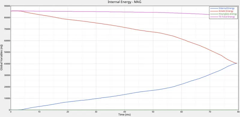
                                                                            fig 5.60

6. Conclusion:

• Bought the center of gravity near to the driver seat.
• Created the sections on cross members.
• Created the intrusions(Springs).
• Gave the initial velocity.
• Gave the connections.
• Created the interfaces.
• Requested for the outputs, by assigning the TH.
• Finally, plotted the results by using various graphs.

7. Learning outcomes:

By doing this challenge, the following aspects can be learned:-

• Balancing the mass to obtain the COG at the required position( By adding the masses).
• Creating the sections.
• Obtaining the intrusions with the help of springs.
• Giving the initial velocity.
• Creating the interfaces.
• Post-processing with the help of obtained values.