Frontal Crash Analysis of a Dodge Neon BIW model using Radioss.

Objective:

To perform the Frontal crash analysis of a Dodge Neon BIW model and study the results.

The following operations need to be performed:

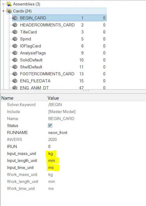
• Check unit system and either follow[Mg mm s] or [Kg mm ms].
• Create appropriate interface ,friction 0.2 and recommended parameters.
• Make sure of no penetrations and intersections are present.
• Correct rigid bodies if any issues.
• Create rigid wall with friction 0.1.
• Compare the model weight with the full scale 300k nodes model and use added masses to reach target weight 700kg while getting CG about the required range.
• Set Initial velocity as 35 mph.
• Use model checker to ensure good quality.
• Set Time-step as :0.5 to 0.1 microseconds.
• Run the simulation for 80 ms.

Output requests:

• Sectional force in the rails at location of indicated node 174247.
• Axial force received on the rails from bumper.
• Shotgun cross sectional forces.
• A pillar cross sectional forces.
• Acceleration curve received on the accelerometer at base of B pillar (on B pillar rocker).
• Intrusions on the dash wall nodes - 66695,66244.

Procedure:

1. Open Hyperworks and import the solver deck that is given.

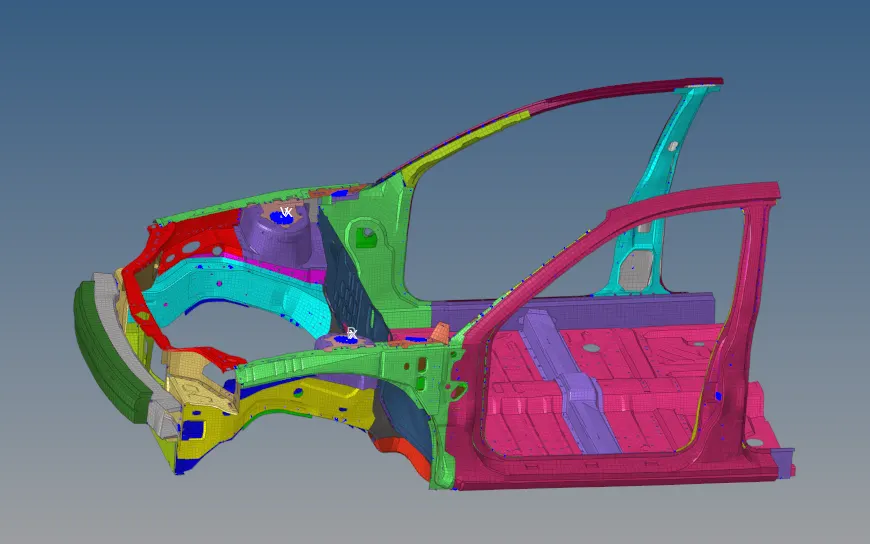
2. The model will look as follows:

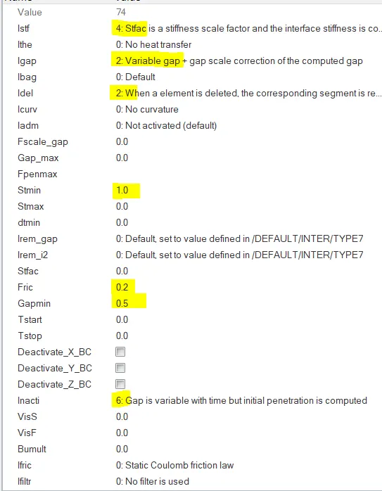
3. The primary check is for the unit system used.

4. Go to BEGIN_CARD in the CARDS deck and check these values as shown below.

5. It is found to follow: kg, mm ,ms.

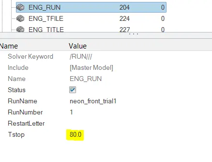
6. Let us next set the Engine Run time.

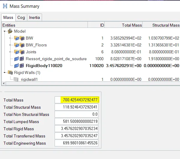
7. Go to the ENG_RUN time card and set the value of Tstop to 80ms

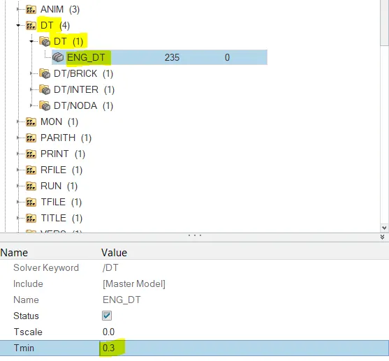
8. Go to ENG_DT in the Solver tab under DT heading and change the value of Tmin to 0.3. (Any value between 0.1 - 0.5)

9. Let us next check for penetrations.

10. Go to tools -> Penetration Check.

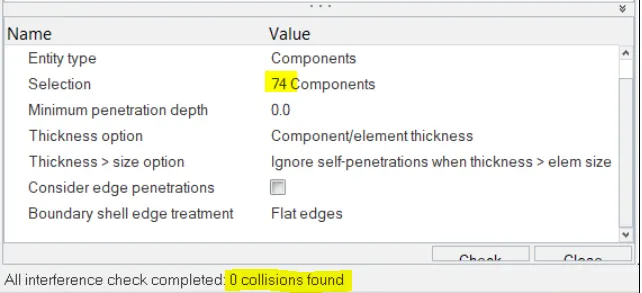
11. Select the components, set the values and hit check.

12. No Penetrations were found as shown below:

13. The next step is to create the Rigid wall.

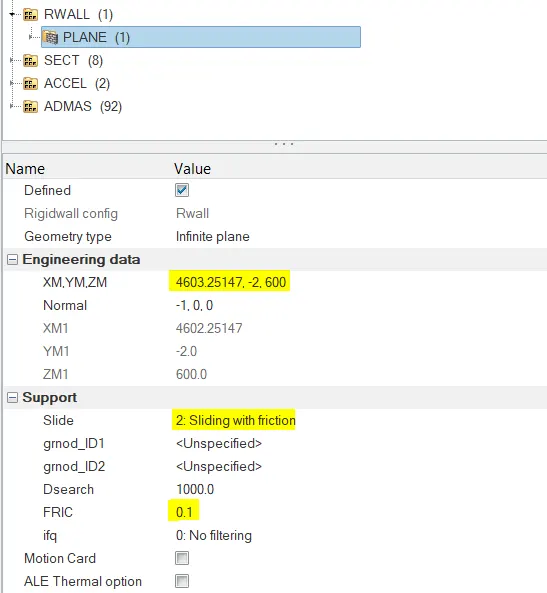
14. Right click in the solver tab -> Create -> RWall -> Infinite Plane.

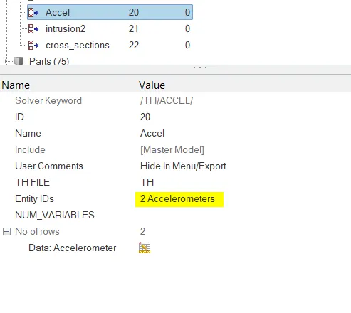
15. Select a node on the bumper to set it as the X point for the wall.

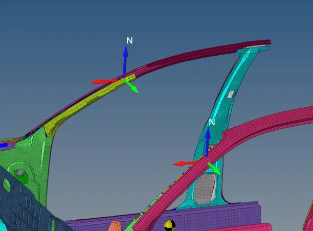
16. Adjust the values such that there is a distance of 10 mm from the wall to the bumper.

17. Set Slide =2 and the value of Friction to be 0.1 as shown below:

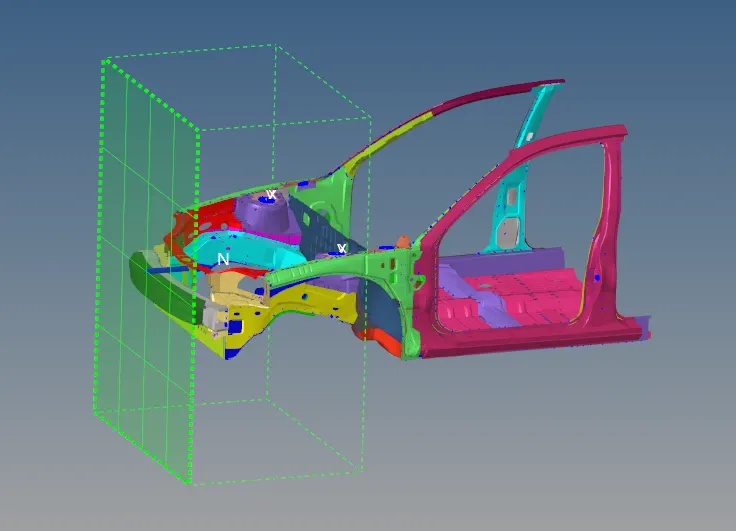
18. The Rigid Wall will look as follows:

19 .Next we move on to setting the velocity.

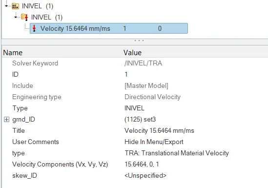
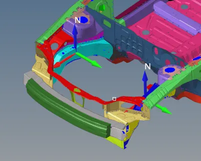
20. The velocity that is required is 35 mph. We convert this to mm/ms to obtain the value of velocity as: 15.6464 mm/ms

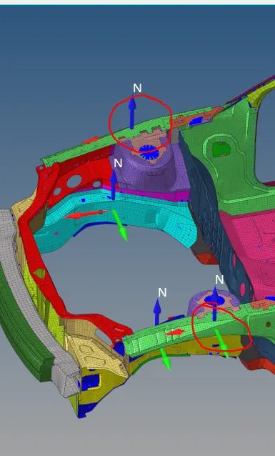
21. To create the INIVEL property, right click on the Solver tab -> Create -> Boundary Conditions -> INIVEL.

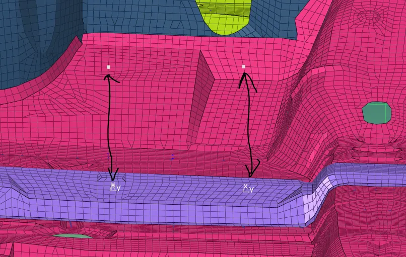
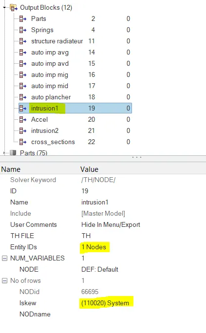
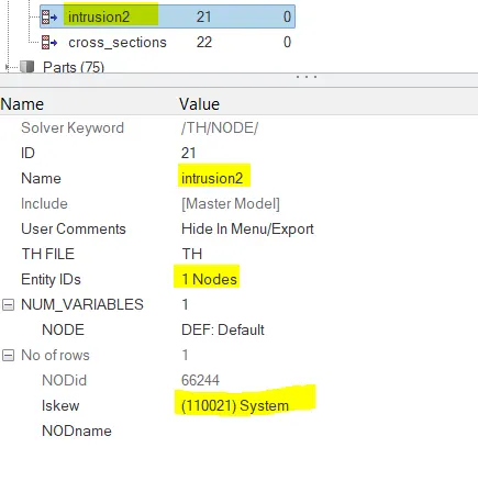
22. All the nodes in the model are selected and a velocity of 15.6464 mm/ms is applied on them as shown below:

23. The next step is to set up connections.

24. Create a new Type7 connection with the recommended properties as shown below and delete the remaining connections that were provided.

25. This will look as follows:

26. Following this, we set the COG and mass of the model as required.

27. As we know, the COG of the BIW of the car is supposed to be at the rear bottom of the driver and passenger seats.

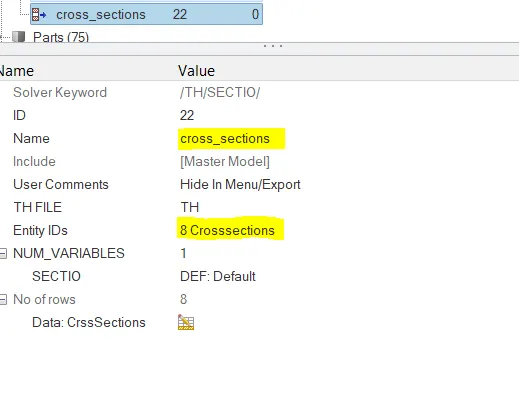
28. To achieve this COG and a target mass of 700kg, we assign masses to the model.

29. This is done by using the ADMAS option.

30. Old COG:

x: 3163.956299623183

y: -2.667949046606327

z: 440.40979420876516

31. New COG after mass addition:

x: 2629.3076952044053

y: 16.94168734215426

z: 291.33428212101313

32: The total mass has also reached the target value of 700kg as shown below:

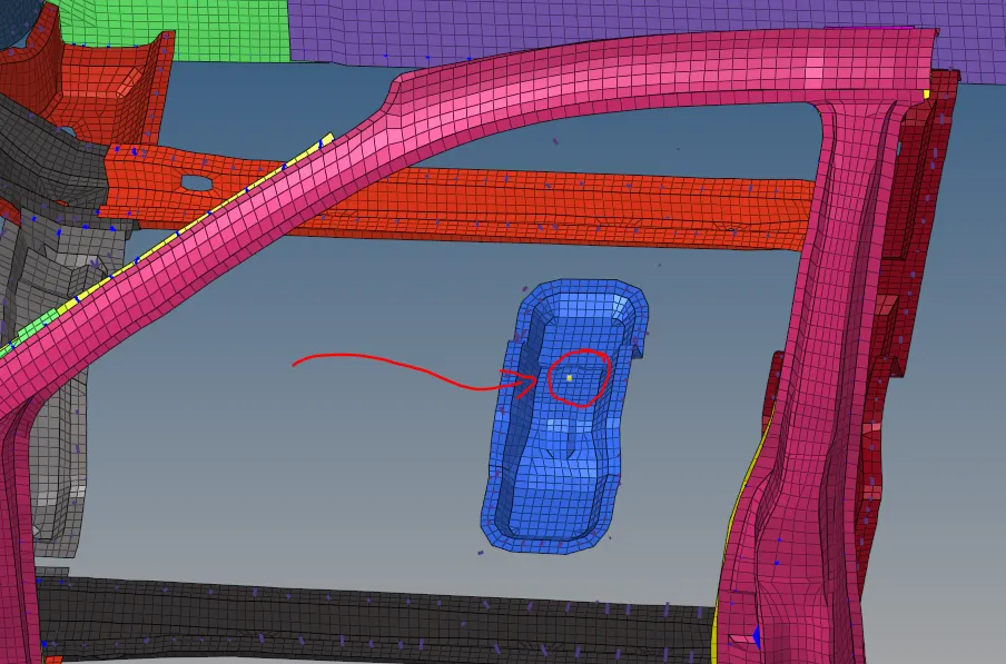
33. The Centre of gravity point in the model:

Output requests:

34. We next move into specifying the output parameters that we want.

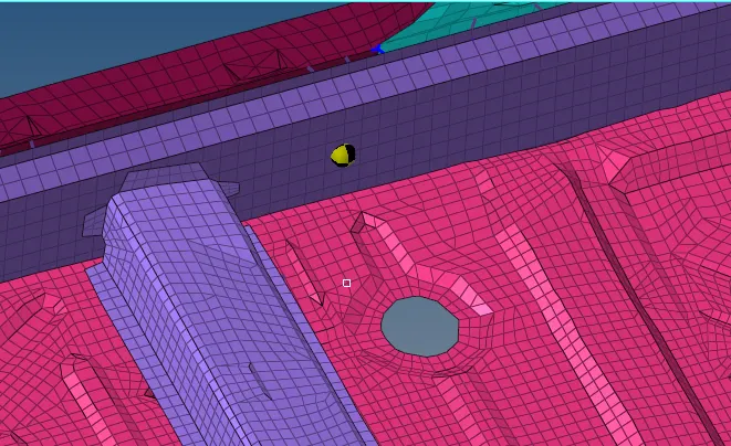
35. Firstly we need to plot the Acceleration curve received on the base of B pillar (on B pillar rocker).

36. For this we place an accelerometer at these two pillars by Right clicking on the Solver tab -> Create -> TH -> ACCEL as shown below:

37. Next we are required to calculate the cross sectional forces on the A pillar.

38. We therefore create a new section by Right clicking on the Solver tab -> Create -> SECT.

39. We create a FRAME if necessary to define the section better and select the nodes and elements as required.

40. The A pillar, after specifying the cross section looks as follows:

41. The same is performed for the rails shown below:

42: Shotgun cross section:

43. Similarly we set up the intrusions on the dash wall at nodes 66695,66244.

44. For this, we set up skews that align in the same line as the nodes mentioned above and select the corresponding skew to measure the intrusion onto the dashboard.

45. This is illustrated below:

46. The next step is to assign the parameters in the output block so that we get a the required outputs.

47. In the output block, the skews are selected as discussed above for both the intrusions:

48. Similarly we set up the output block of the accelerometers as shown below:

49. We set up the output block for the Cross- Sections as shown below:

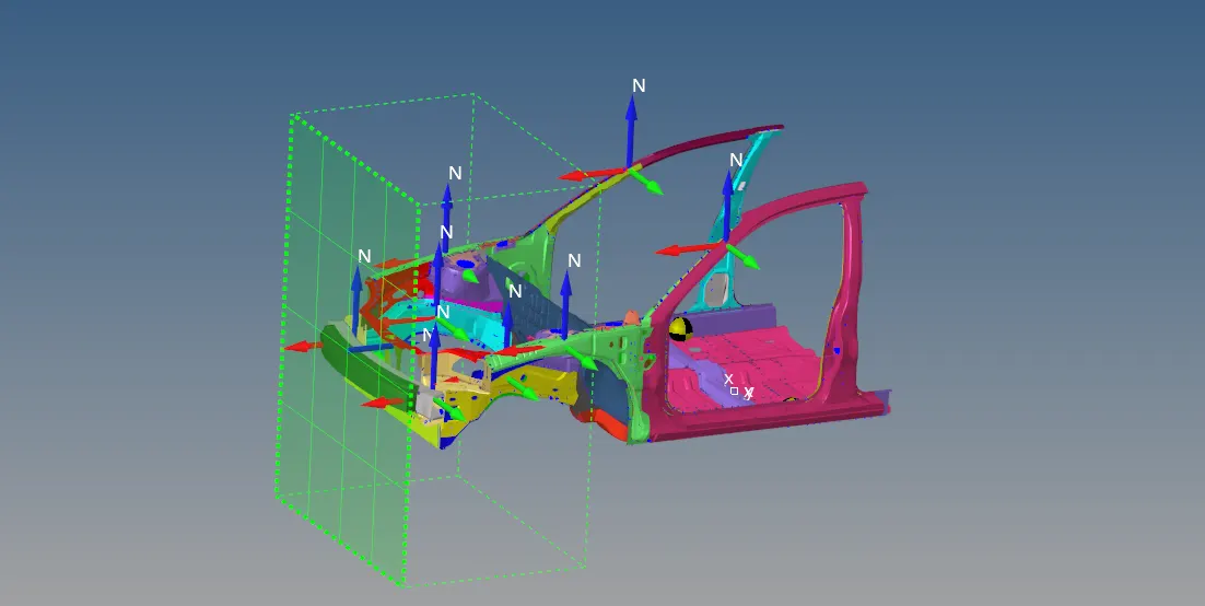
50. The final model will look like this:

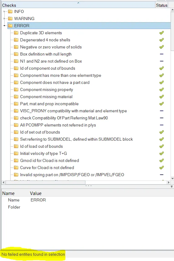
51. Go to Tools -> Model Checker and run the Errors and Warnings and check if any Errors are present and fix them.

52. No errors occurred as shown below and hence the model is ready to run.

53. Go to Analysis -> Radioss and set the options to -nt 4 and run the simulation by clicking the Radioss button.

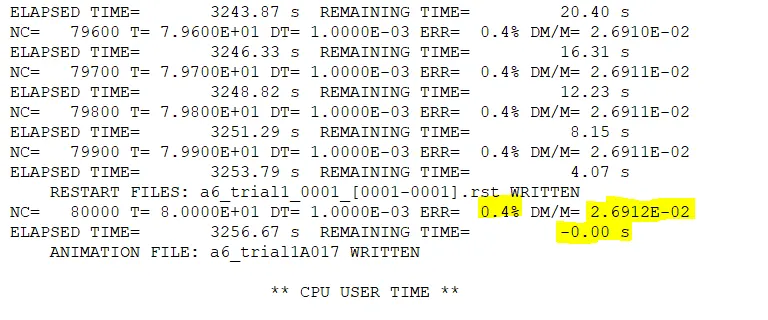
54. The Energy and Mass error are within the given limits and hence we can move forward.

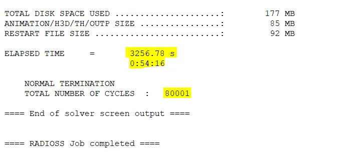
55. The Simulation time was 54 mins 16 s and the total number of cycles were 80001.

Animations:

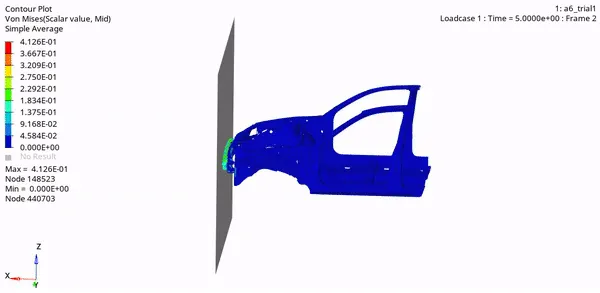
56: Von Mises Contour Plot:

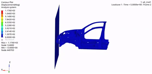
57. Displacement Contour Plot:

58. Swtich to Hypergraph and open the T01 file.

59. Plot the required graphs to analyse the results.

Results and Conclusions:

Global Variables:

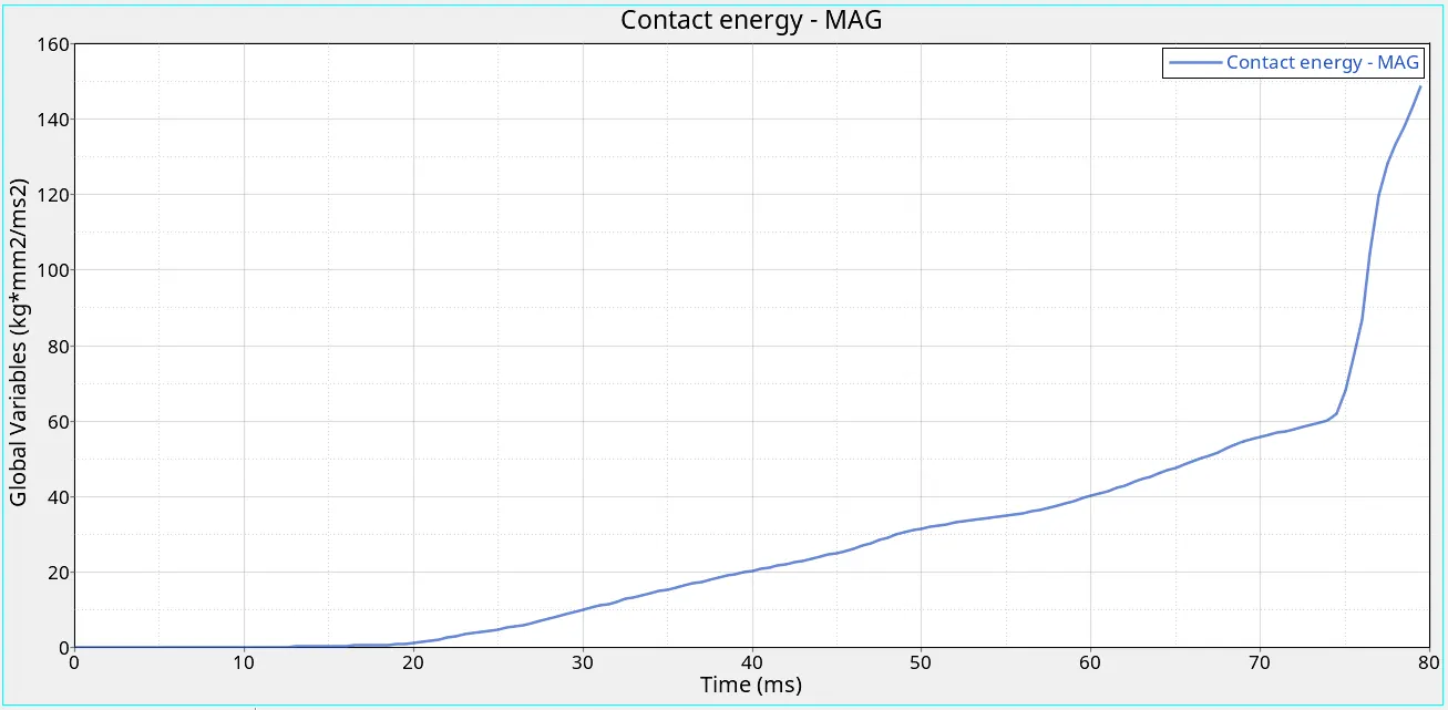
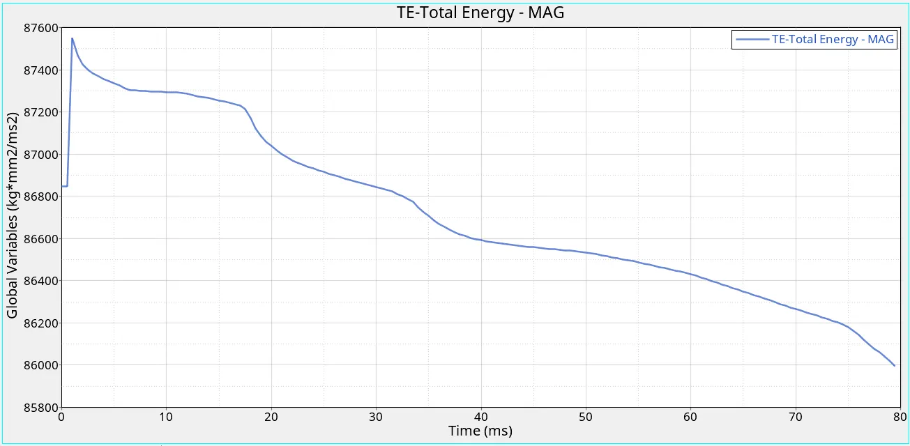
The grpah below shows Internal Energy. Kinetic Energy, Hourglass energy, Contact energy, Total Energy and Total Translational Energy vs Time.

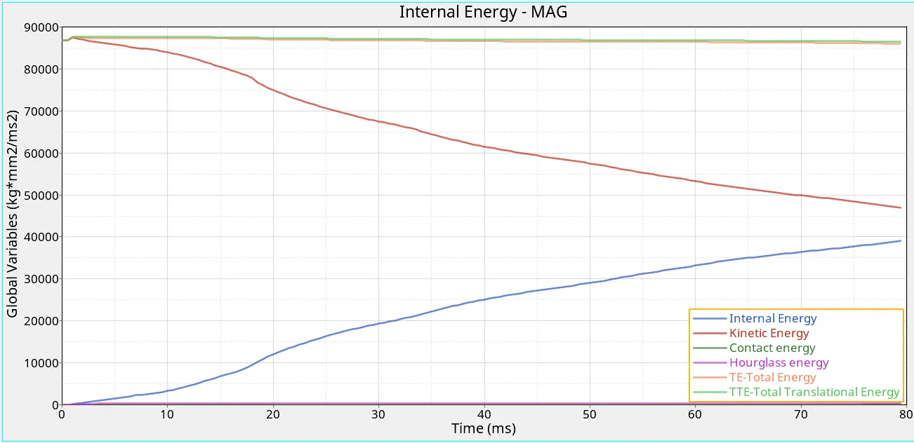
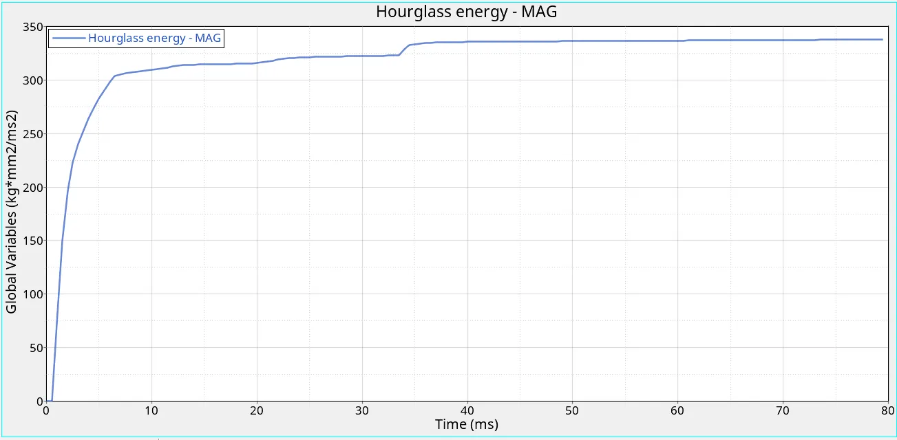
• We see a constant dip in Kinetic energy and a constant increase in Internal energy.
• At 80ms, both these values are in the ~ 40000 - 48000 kg*mm2/ms2 range.
• Hourglass energy reaches a peak value of ~340 kg*mm2/ms2 towards the end of the simulation.
• Contact energy reaches a peak value of 150 kg*mm2/ms2 which is very low comparitively.
• Total energy peaks at around 1 ms with a value of 87550 kg*mm2/ms2 where the impact takes place and decreases rapidly to 86000 kg *mm2/ms2.

Acclerometer graphs:

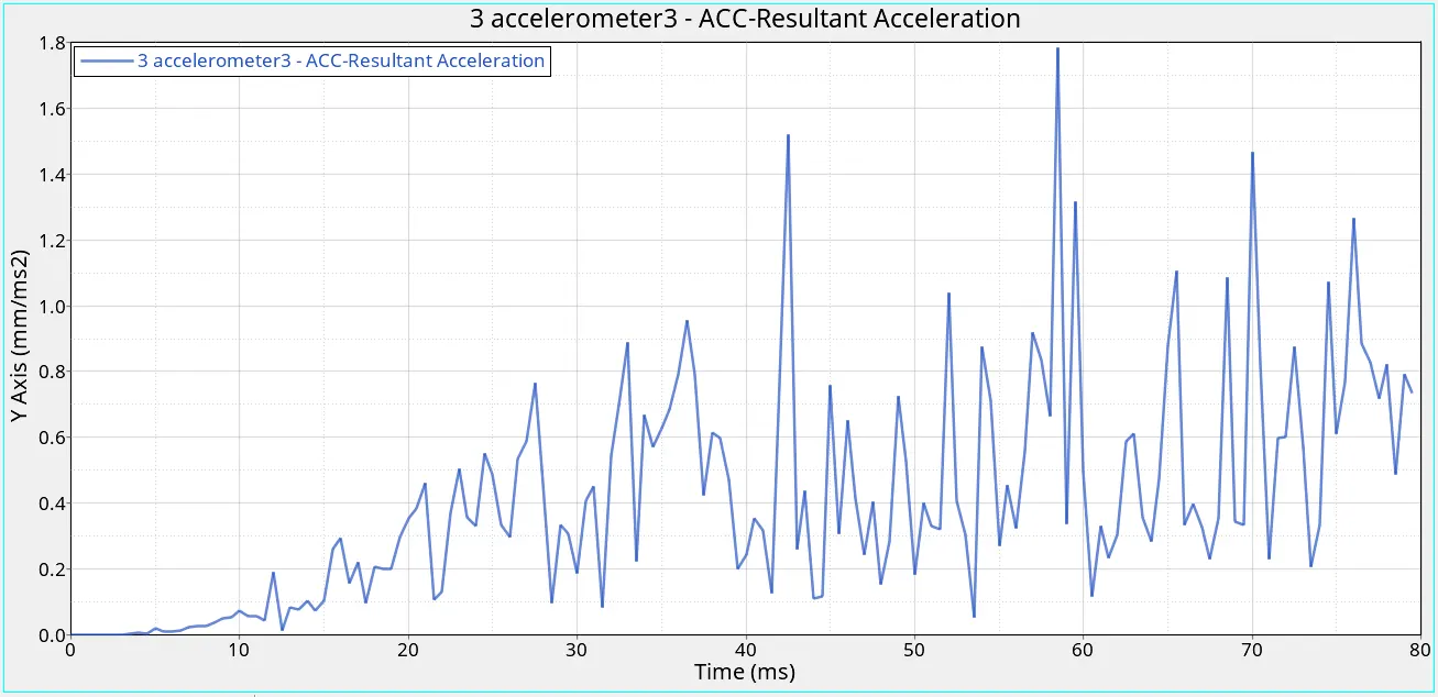
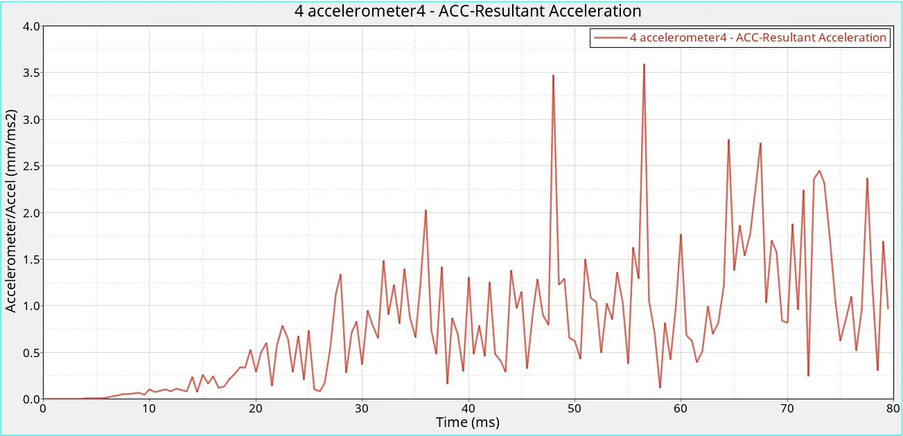
• The accelerometer graphs show many peaks throughout the simulation

Intrusions (Displacement):

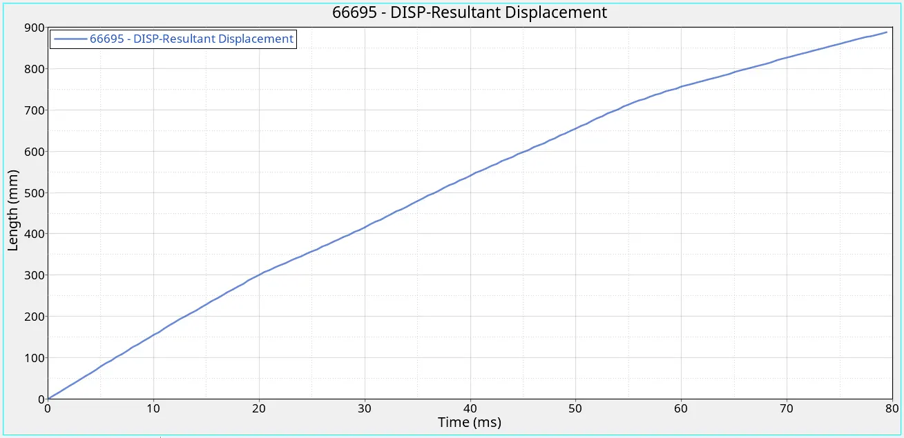
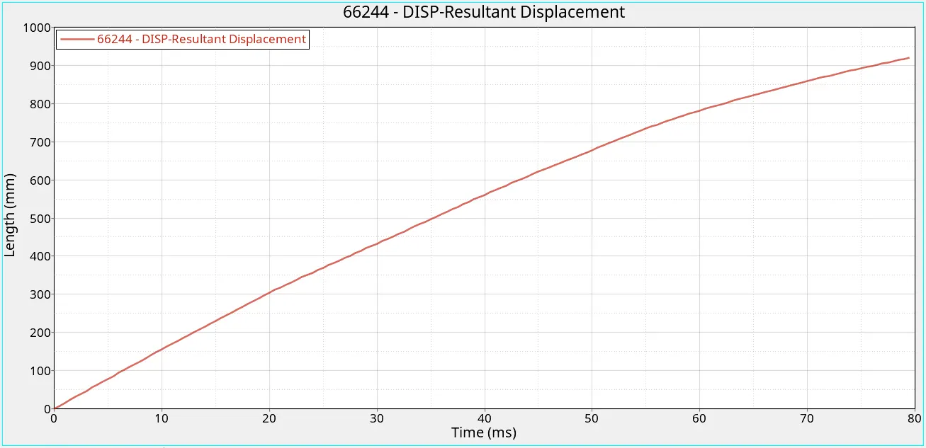
• The above graphs show the plots for displacement from the centre pillar to the dashboard.
• The maximum value ~ 900 mm is reached towards the end of the simulation at around 79 ms.
• This is a good sign because the later the maximum value is reached, the better force absorption characteristics.

Plots for the Cross-sectional forces:

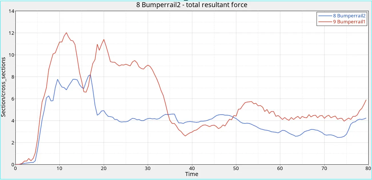
Bumper-rail:

Hinge Rail:

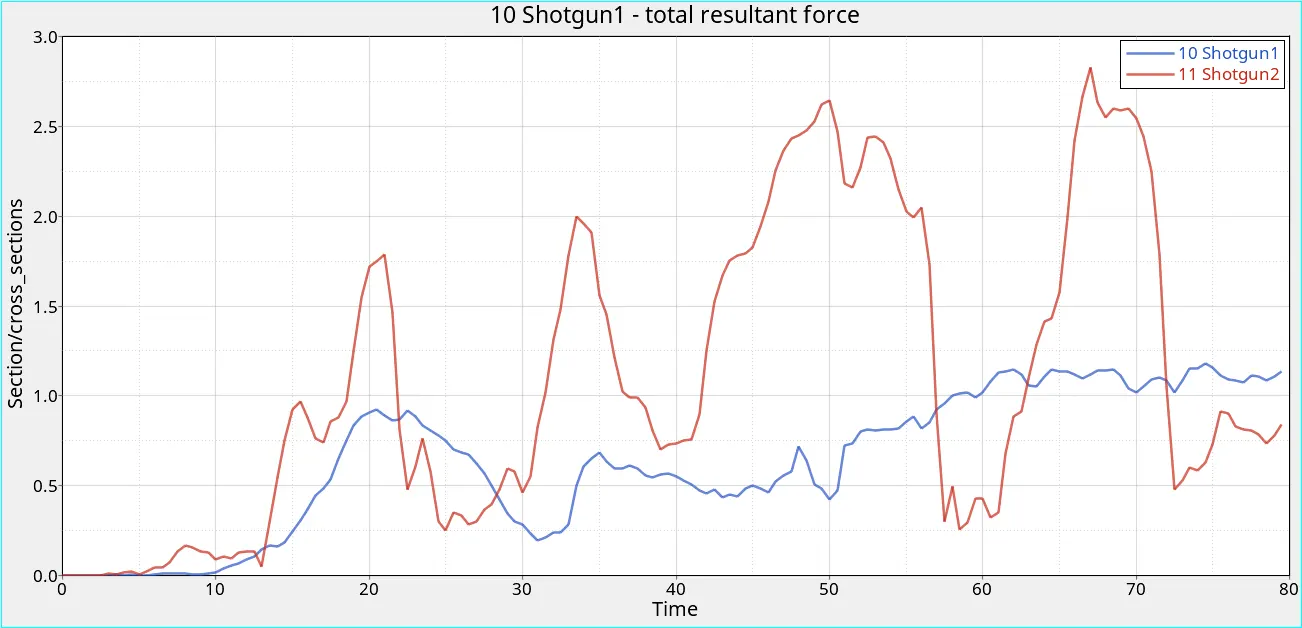
Shotgun:

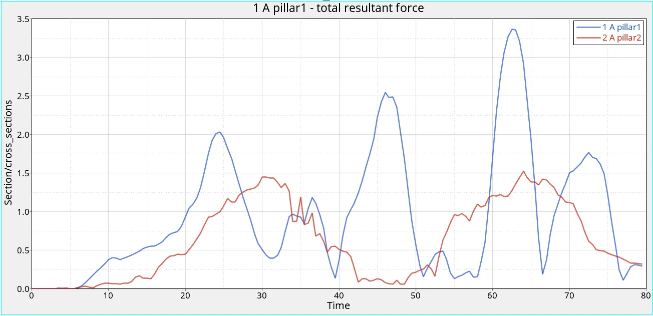
A pillar:

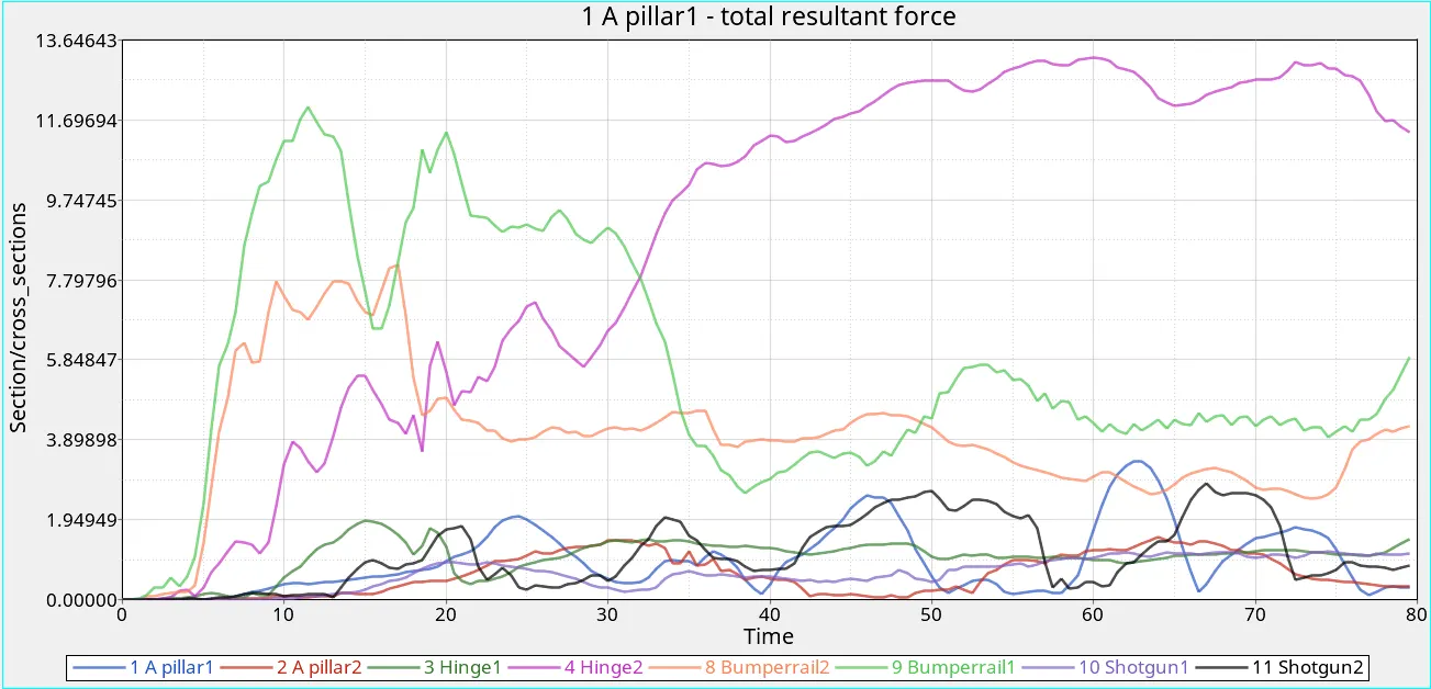
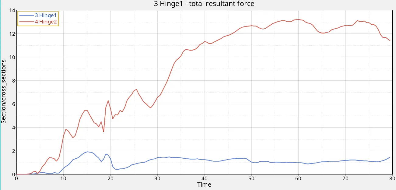
From the above graphs we notice that:

• The maximum force at Bumper rail is 12 kN at ~ 11 -12 ms.
• The maximum force at the Hinge rail cross section is 13 kN at ~ 60 ms.
• The maximum force at the Shotgun cross section is 2.75 kN at ~ 68 ms.
• The maximum force at the A pillar cross section is 3.4kN at ~ 62 ms.

Conclusions:

• From these results we get an idea as to how these designs need to be modified.
• The Bumper Rail and Hinge experience the highest amount of force ~ 12 -13 kN. Therefore the geometry and material selection for these parts are critical since they have the highest probability of failure.
• The Shotgun and A pillar experience maximum loads of 2.75 and 3.4 kN, however, the A pillar is a critical component that is essential for a safe crash scenario.
• If the loads on the A pillar or any other critical component is too high, adjustments can be made to the design such that the forces are well distributed and not concentrated on the critical components.