Analysis and Comparison of Different Contact Interfaces and Notch Significance on a Crush Tube Model using Radioss.

Objective:

• To Mesh the given bumper model with an element size of 6mm.
• To run the given crash tube model with different conditions under 6 different cases:
  1. Run the crash tube as it is
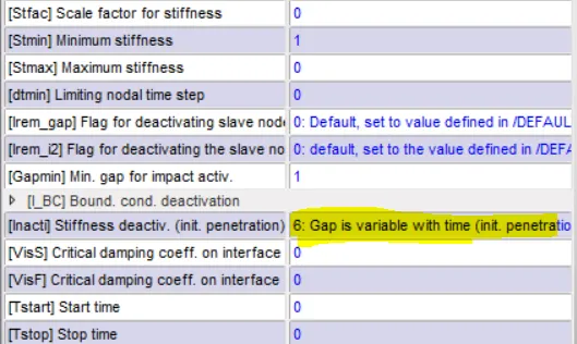
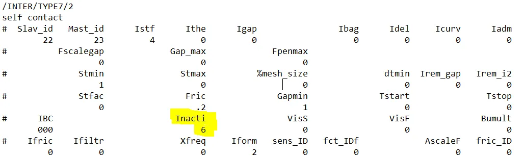
  2. Change the Inacti = 6 and run
  3. Create Type 11 contact and run
  4. Remove both the notches and remove boundary conditions on the rigid body and then run.
  5. Create a new notch in the middle, select the whole section and run.
  6. Create a new notch with nodes only from opposing 2 faces and run.

Procedure:

Meshing the given model:

1. Open the given hypermesh model.

2. First we fix the given model for any free edges.

3. These free edges can be fixed using the Extend surface command in the surface edit panel.

4. After extending, the surface will have a green line to show that it is connected to another surface.

5. The yellow line indicates that the side is shared by more than 2 surfaces.

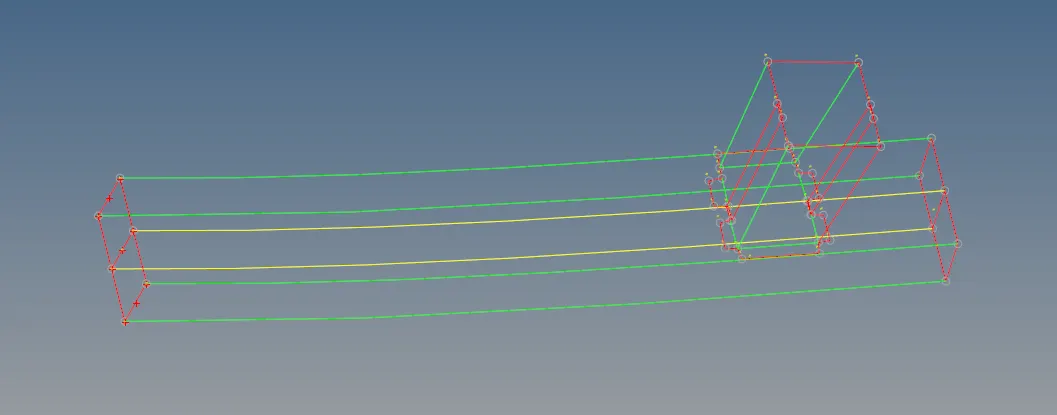
6. The next step is to mesh the surfaces.

7. Go to f12(automesh) -> set the element size to 6 -> select the surfaces -> enable align and size -> hit mesh.

8. If there are any trias formed, it can be removed by changing the number of elements in the edge.

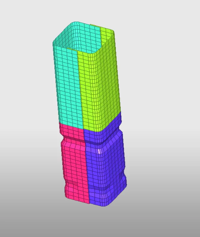
9. The final meshed geometry will look as shown:

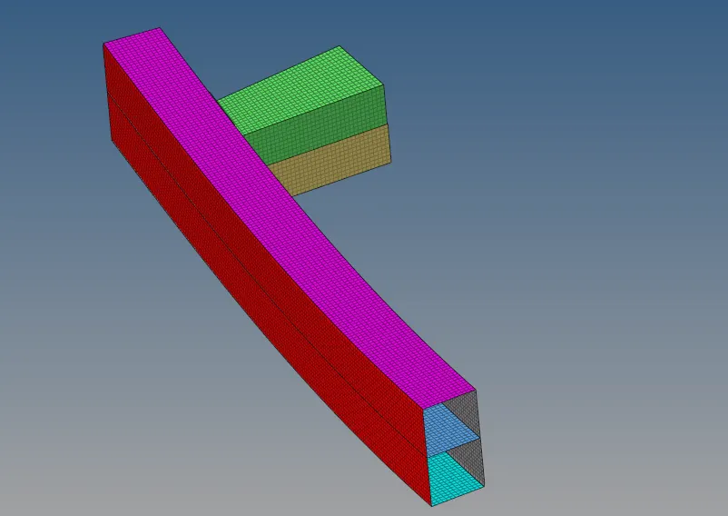
10. Check the model for quality and make sure that the elements dont deviate much from the target element size:

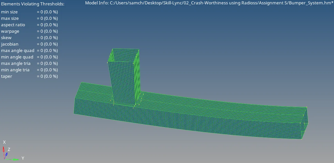
11. The final model looks as follows:

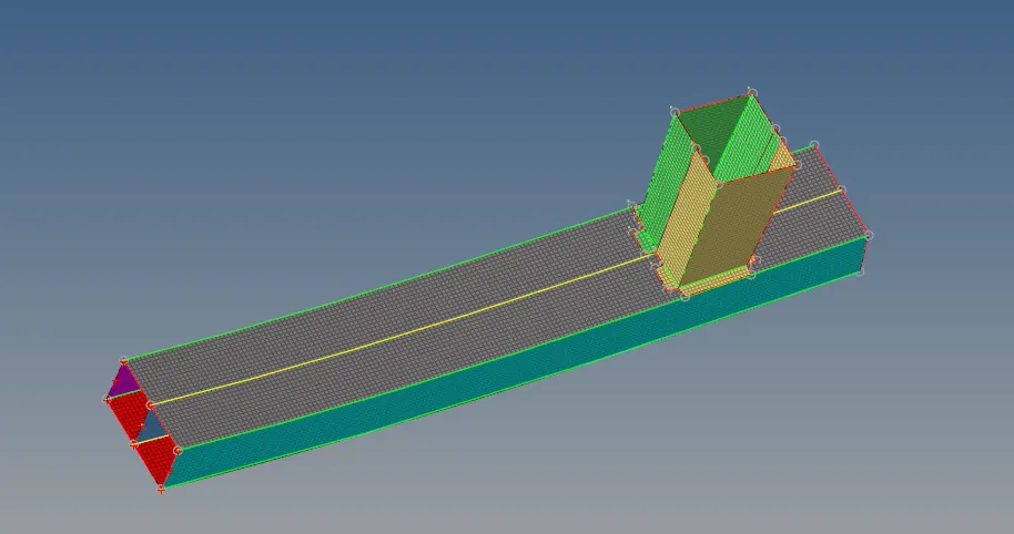
Crush tube Simulation:

Case 1: Run the model as it is.

1. Open Hyperworks and go to Import Solver Deck and import the given solver deck Crush_tube_0000.rad.

2. The model will look as shown below:

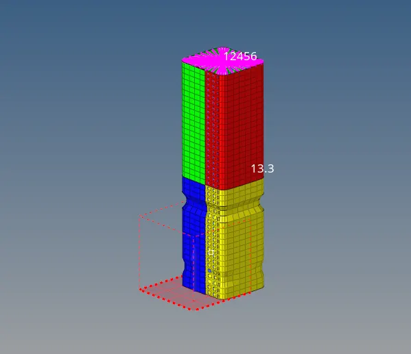
3. Go to Analysis -> Radioss and run the model with options set to -nt 4.

4. Hyperworks Solver view will show the following:

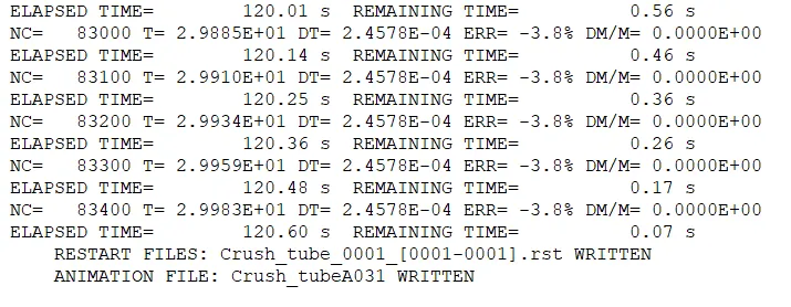
5. From this we see that the Energy error and Mass error within the allowable limit and hence we can move forward with the simulation and view the results.

6. Open the results file. Open .h3d file to view the animation and .T01 to plot the required values.

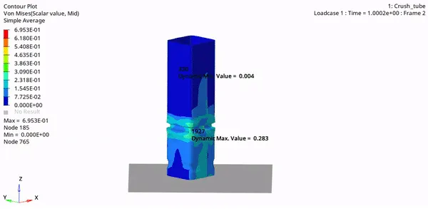
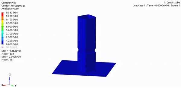
7. Animation:

Von Mises Stress:

Contact Forces:

8. The following graphs are plotted:

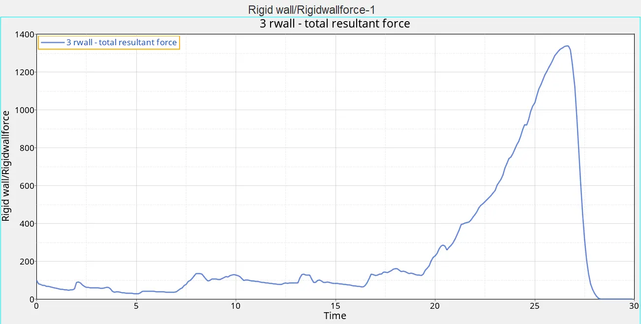
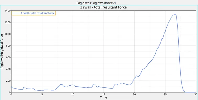
Rigid wall force (total resultant force):

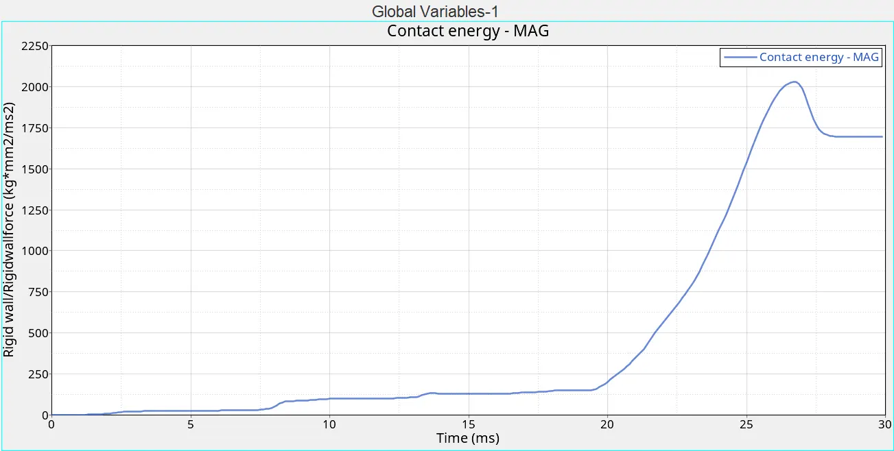
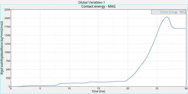
Contact Energy:

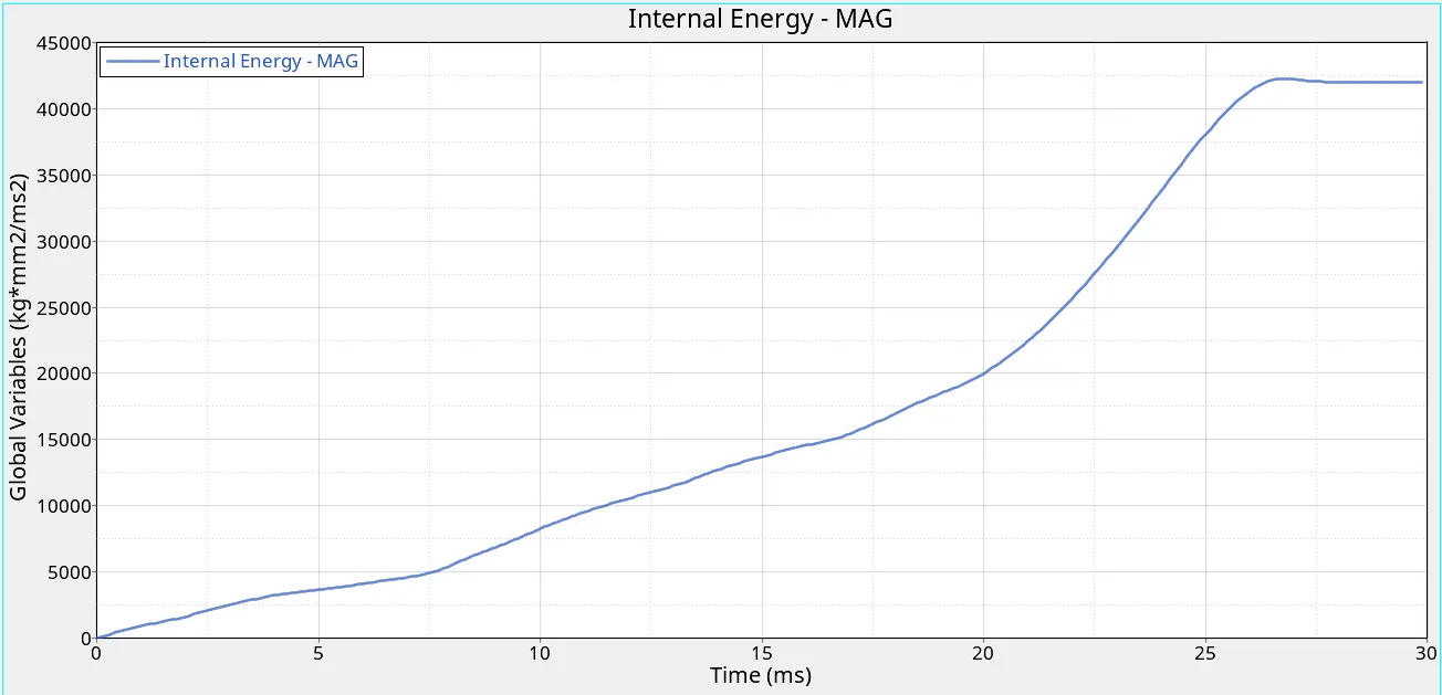
Internal energy:

Case 2: Change the Inacti = 6 and run

1.Continue on the same model.

2.Change the value of Incati = 6 as shown below:

3. Export the Solver deck and open the file in Notepad to check whether the changes have been made.

4. Run the simulation using Radioss and check the solver view as shown below:

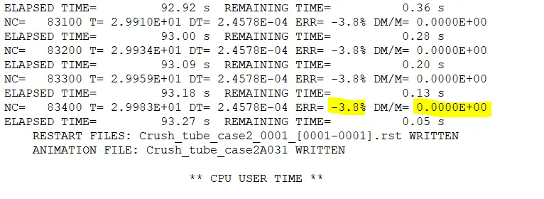
5. From this we see that the Energy error and Mass error within the allowable limit and hence we can move forward with the simulation and view the results.

6. Open the results file. Open .h3d file to view the animation and .T01 to plot the required values.

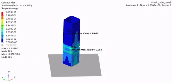
7. Animation:

Von Mises Stress:

Contact Forces:

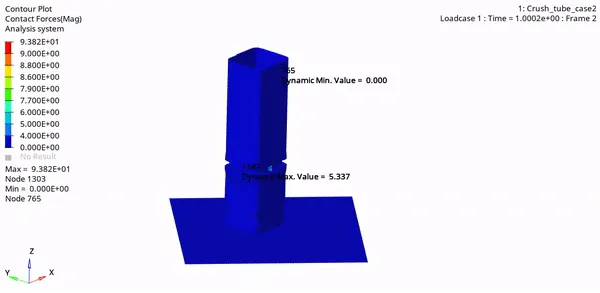
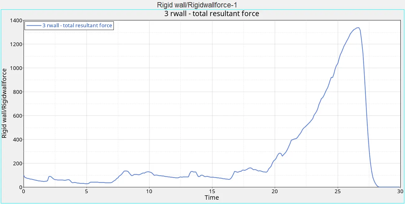
The following graphs are plotted:

Rigid wall force (total resultant force):

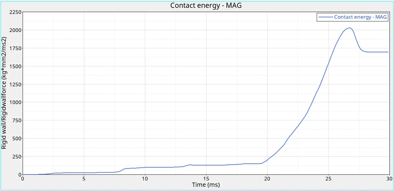
Contact Energy:

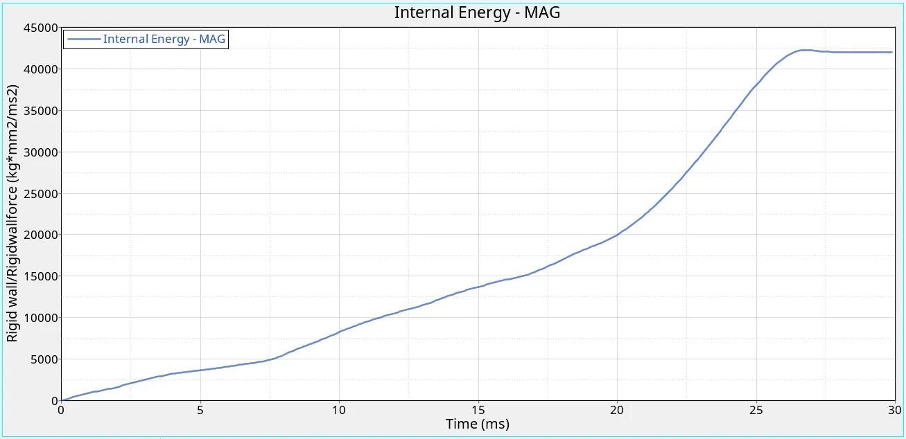
Internal energy:

Case 3: Create Type 11 contact and run

1. Continue on the same model.

2. Go to the tree on the left side and go to groups.

3. Right click and create a new contact and name it Type11.

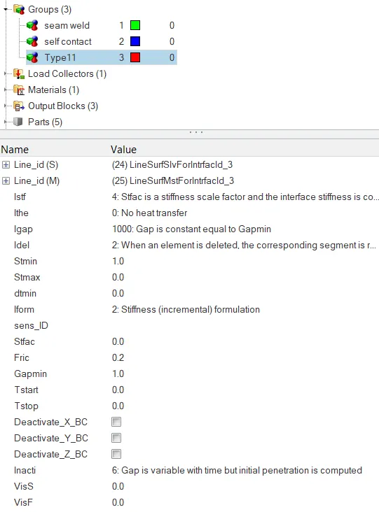
4. Set the values as shown below and continue to export and run the simulation on Radioss.

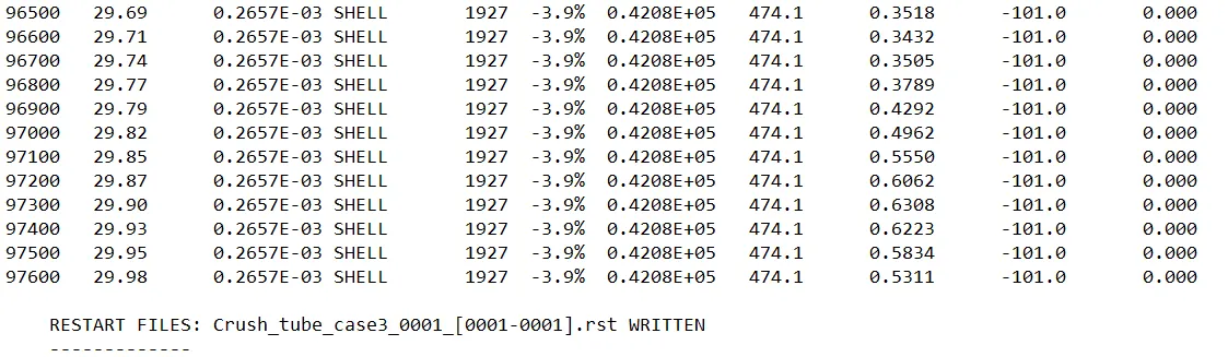
5. We see that the Energy error and Mass error within the allowable limit and hence we can move forward with the simulation and view the results.

6. Open the results file. Open .h3d file to view the animation and .T01 to plot the required values.

7. Animation:

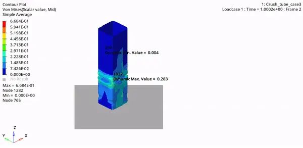
Von Mises Stress:

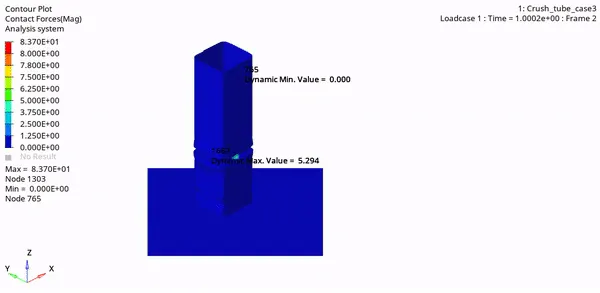
Contact Forces:

The following graphs are plotted:

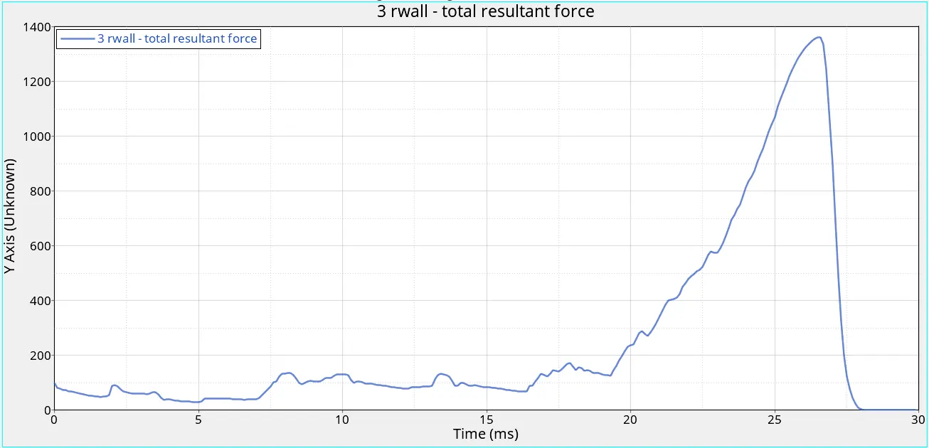
Rigid wall force (total resultant force):

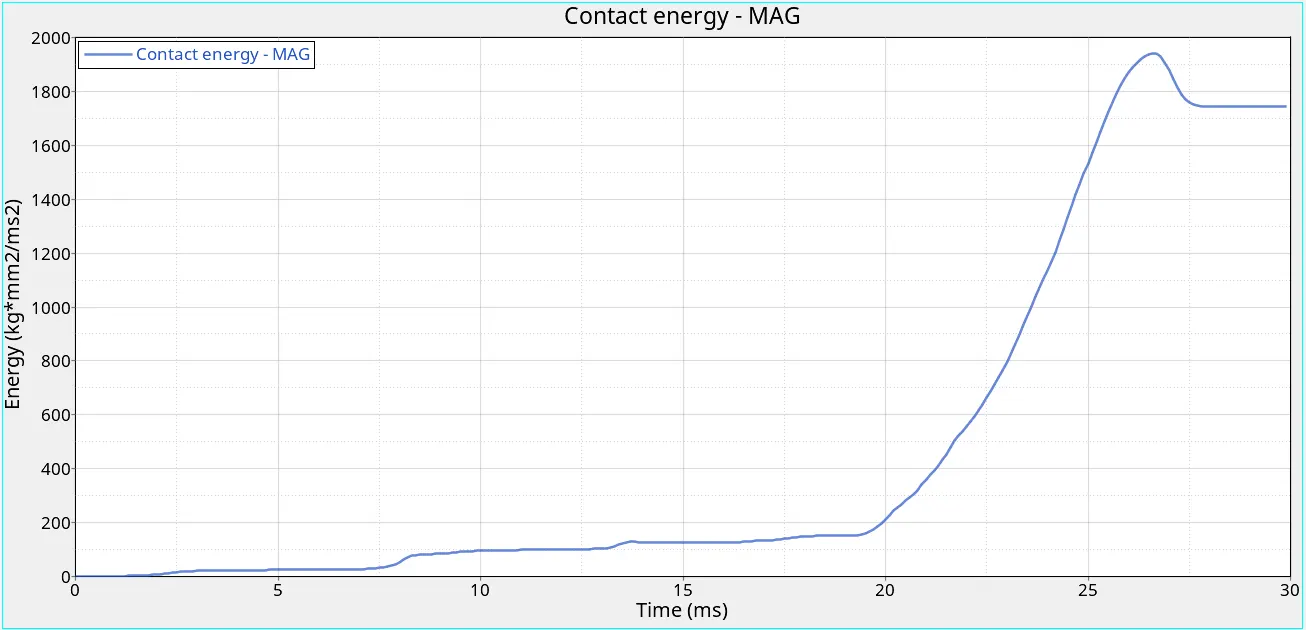
Contact Energy:

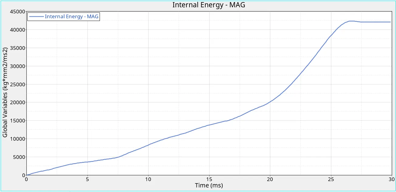
Internal energy:

Case4: Remove both the notches and remove boundary conditions on the rigid body and then run.

1. Continue on the same model.

2. Use the Align tool in Hypermesh to align nodes in such a way that the notches are removed from the model.

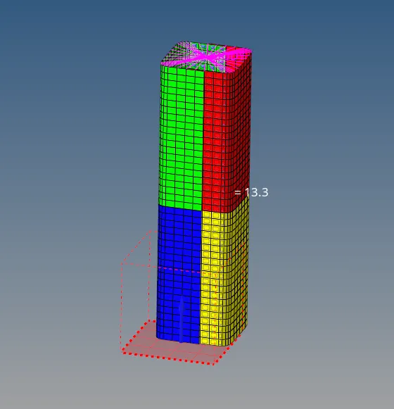
3. Export the Solver deck and save it as a .rad file.

4. The the simulation using radioss. The solver will show the following:

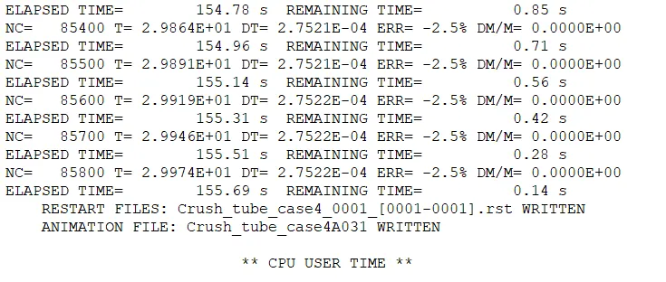
5. From this we see that the Energy error and Mass error within the allowable limit and hence we can move forward with the simulation and view the results.

6. Open the results file. Open .h3d file to view the animation and .T01 to plot the required values.

7. Animation:

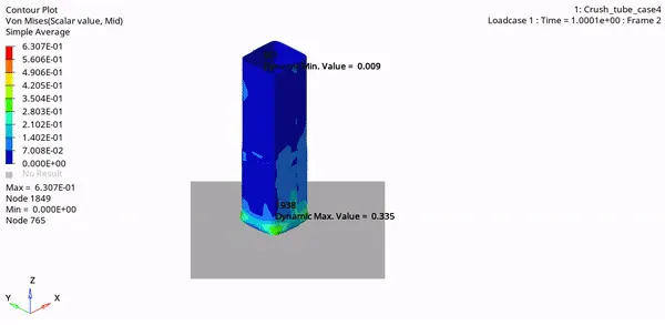
Von Mises Stress:

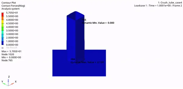
Contact Forces:

The following graphs are plotted:

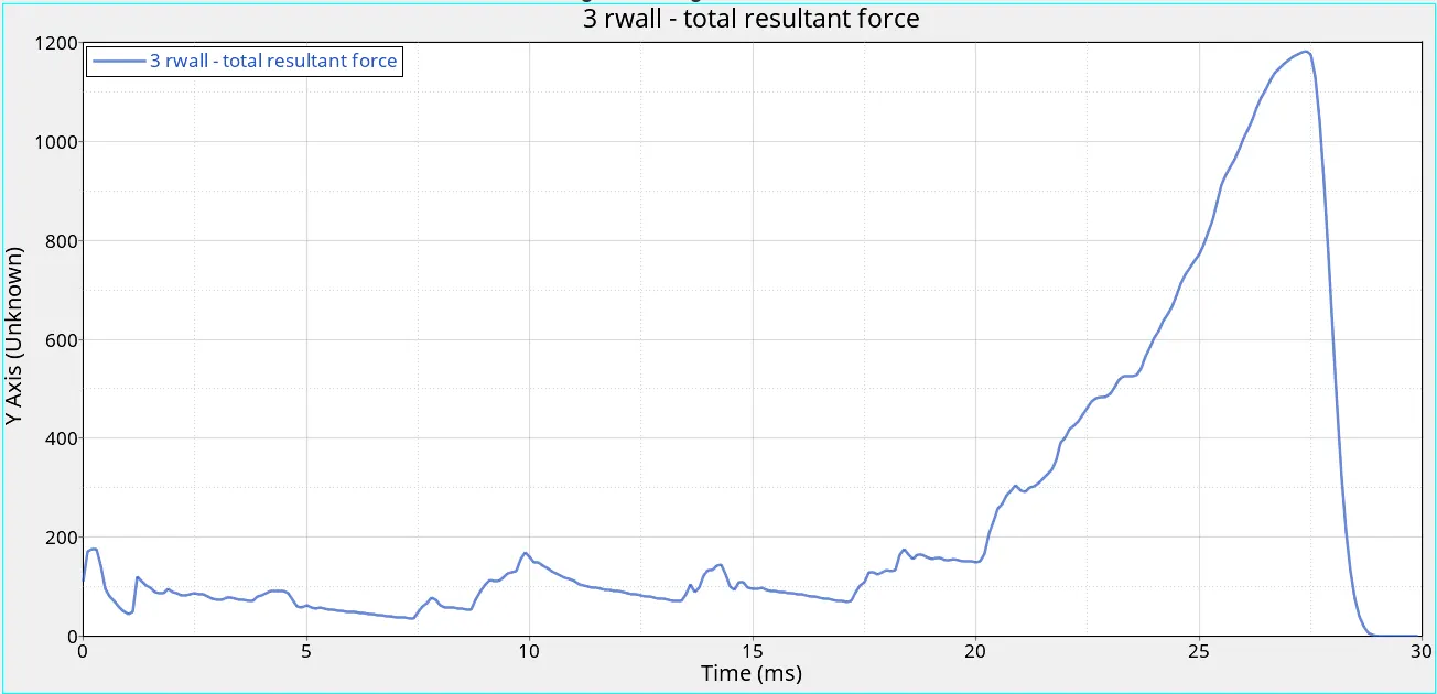
Rigid wall force (total resultant force):

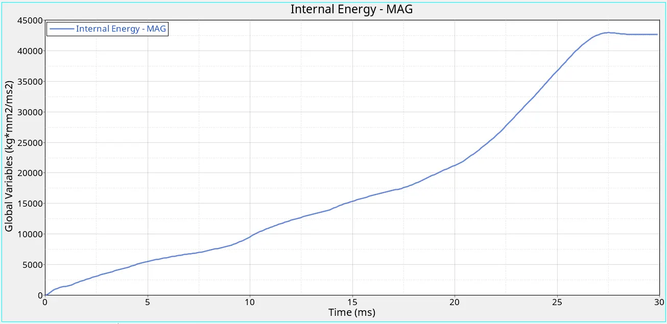
Internal energy:

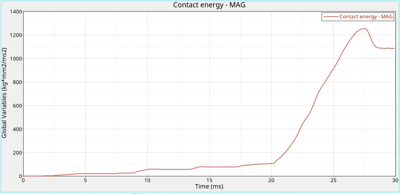
Contact Energy:

Case 5: Create a new notch in the middle, select the whole section and run.

1. Continune on the same model.

2. Remove create a new notch in the middle of the geometry as shown below using the translate command.

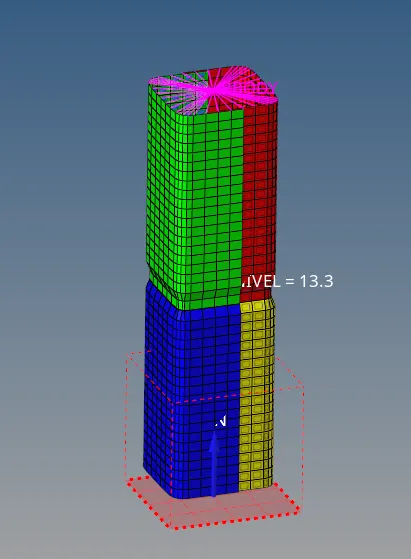
3. Keep all the other setting the same and Export the Solver Deck.

4. The solver will run and show the following:

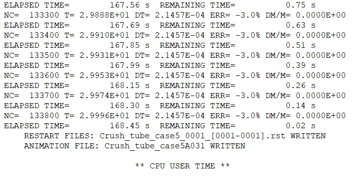
5. From this we see that the Energy error and Mass error within the allowable limit and hence we can move forward with the simulation and view the results.

6. Open the results file. Open .h3d file to view the animation and .T01 to plot the required values.

7. Animation:

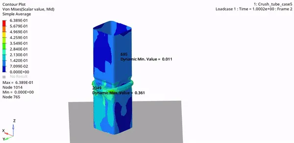
Von Mises Stress:

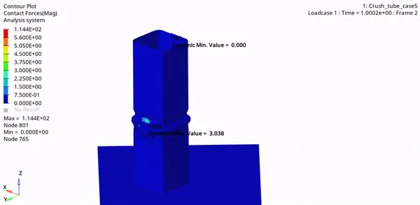
Contact Forces:

The following graphs are plotted:

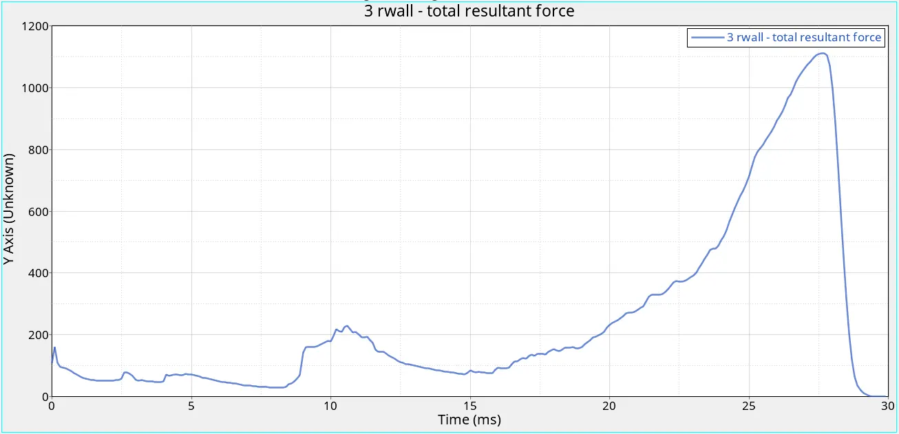
Rigid wall force (total resultant force):

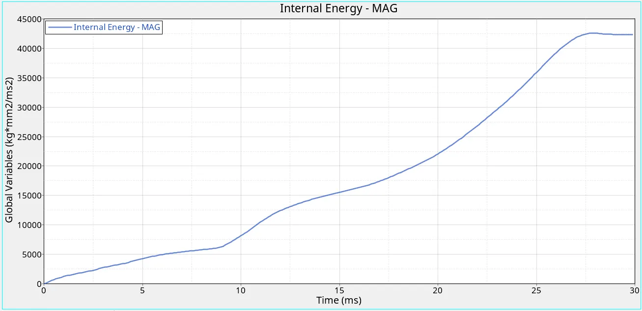
Internal energy:

Contact Energy:

Case 6: Create a new notch with nodes only from opposing 2 faces and run.

1. Continue on the same model.

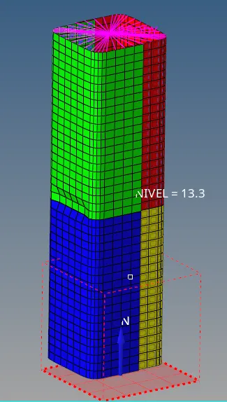
2. Use the align option to create notches on only 2 opposide flat faces of the model.

3. The model should look like this:

4. Export the solver deck and run the simulation using Radioss. The Solver will show the following:

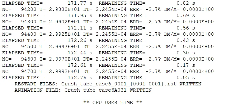
5. From this we see that the Energy error and Mass error within the allowable limit and hence we can move forward with the simulation and view the results.

6. Open the results file. Open .h3d file to view the animation and .T01 to plot the required values.

7. Animation:

Von Mises Stress:

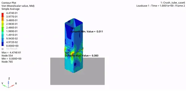
Contact Forces:

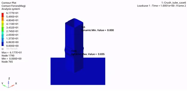
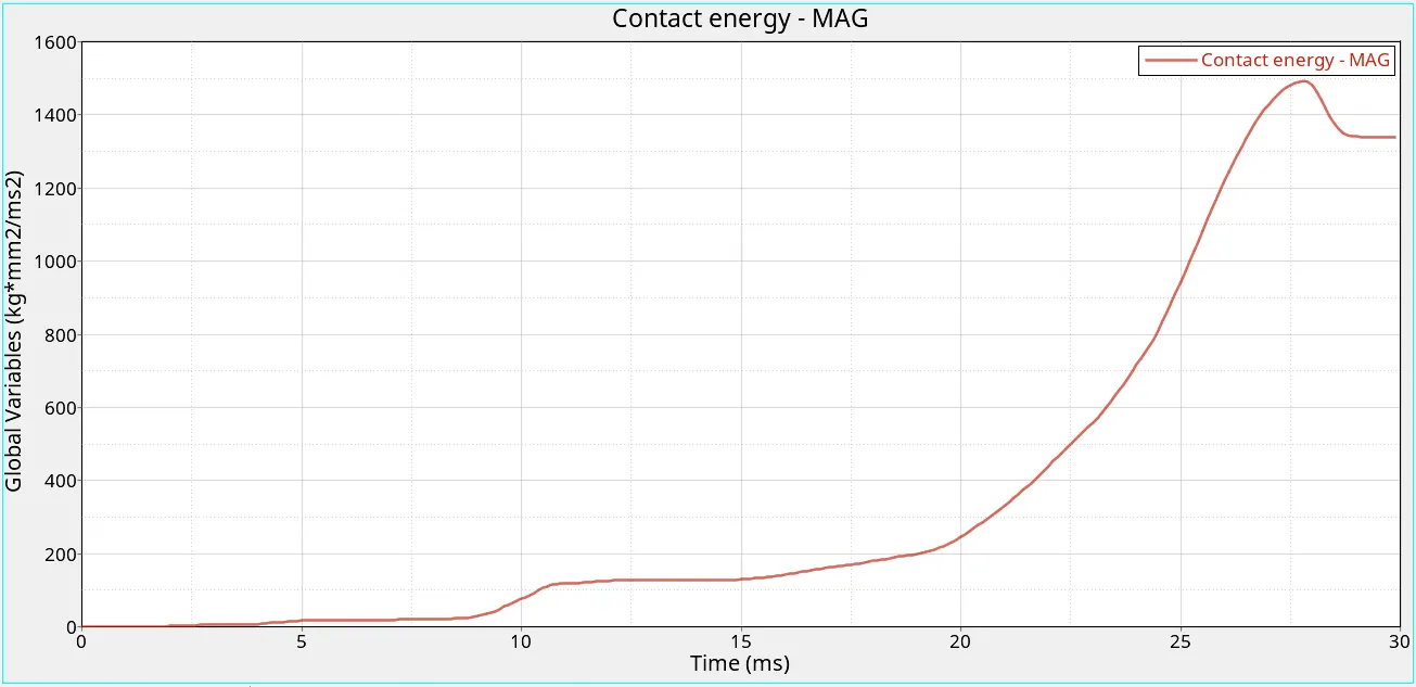
The following graphs are plotted:

Rigid wall force (total resultant force):

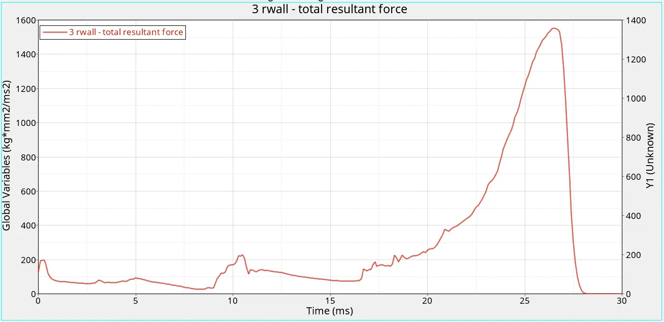
Internal energy:

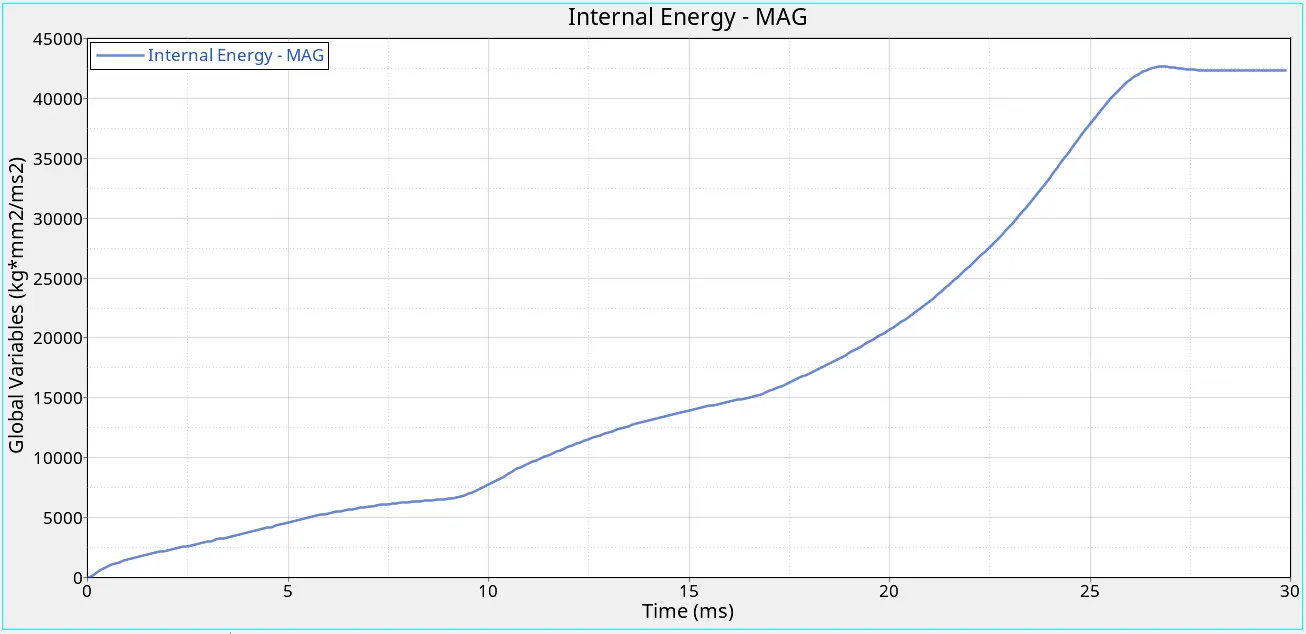
Contact Energy:

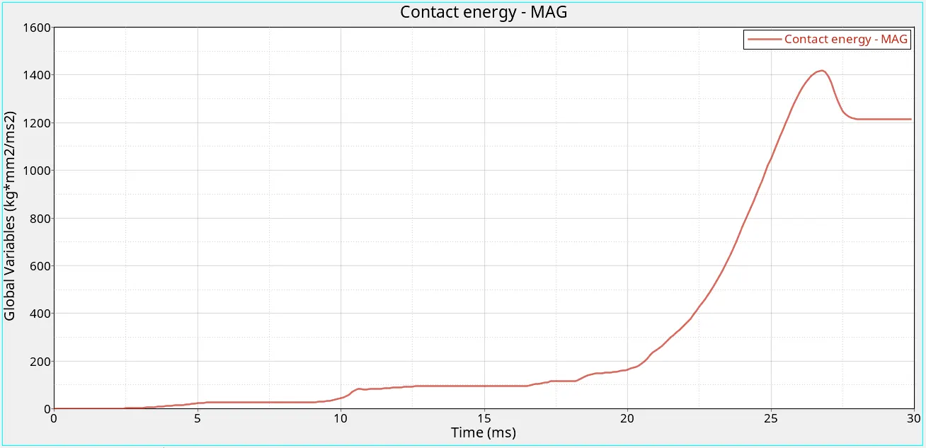
Results and Conclusions:

Comparison of Number of Cycles, Energy and Mass Error and Simulation time:

Parameter	Case 1	Case 2	Case 3	Case 4	Case 5	Case 6
Number of Cycles	83469	83469	97683	85897	133821	94737
Energy Error	-3.8%	-3.8%	-3.9%	-2.5%	-3.0%	-2.7%
Mass Error	0	0	0	0	0	0
Simlation Time	120.70	93.37 s	139.11 s	155.91 s	168.53 s	172.87 s

Conclusions:

• The number of cycles is the highest in case 5 and lowest in cases 1 and 2.
• We see a lower simulation time in case 2 which has Inacti as 6. Inacti =6 reduces the Gap between the slave and master nodes if they go below the calculated Gap.
• The energy error is the highest negative in case 3 and lower negative in case 4.

Comparison of Von Mises and Contact Force animation:

Case	Von Mises	Contact Force
1	Max Von Mises Stress: 69.5 at node 185	Maximum Contact Force : 93.8 kN at node 1303
2	Max Von Mises Stress: 69.5 at node 185	Maximum Contact Force : 93.8 kN at node 1303
3	Max Von Mises Stress: 66.8 at node 1282	Maximum Contact Force : 83.70 kN at node 1303
4	Max Von Mises Stress: 63 at node 1849	Maximum Contact Force : 57.05 kN at node 1020
5	Max Von Mises Stress: 63.8 at node 1014	Maximum Contact Force : 114.4 kN at node 801
6	Max Von Mises Stress: 63.2 at node 775	Maximum Contact Force : 61.7 kN at node 1790

Conclusions:

• The Maximum Von Mises Stress is observed in Cases 1 and 2. This may be due to the notches that are present in the model, which are either removed, or reduced in number in the other cases.
• The Maximum contact forces are found in case 5 followed by case 1 and 2. This is due to
• The Least value of Von Mises stress and Contact force is observed in Case 4 with no notch. So the notch plays a huge role in creating higher stress and forces.

Comparison of Graphs:

Case	Internal Energy	Contact energy	Rigid wall Forces (total resultant)
1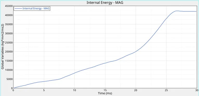
2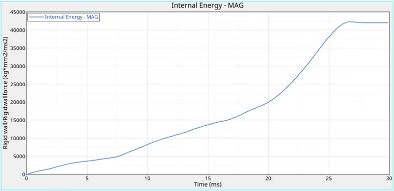
3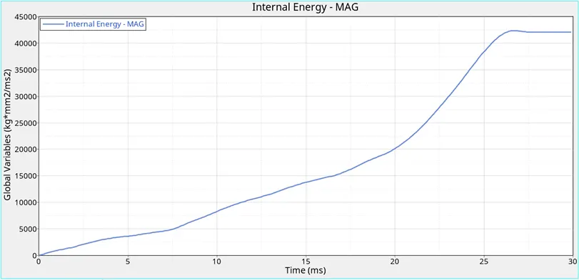
4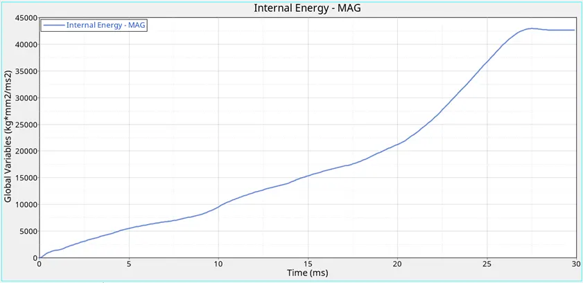
5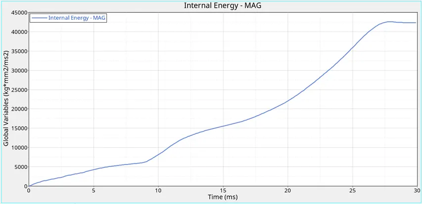
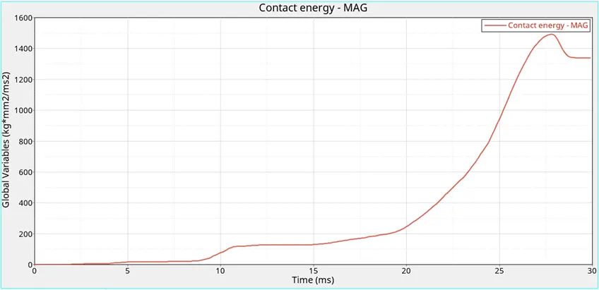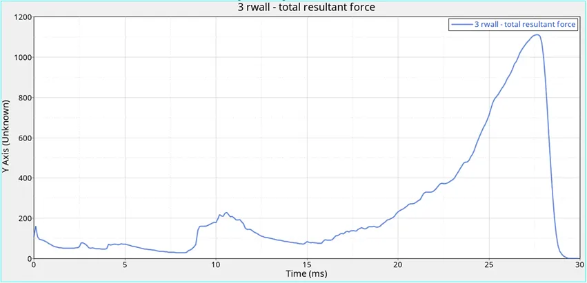6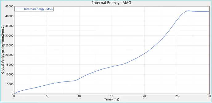

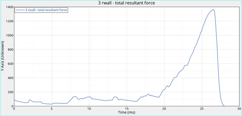
Conclusions:

• Internal energy:
  • For the models with notches, the internal energy graph shows a smoother curve whereas the other cases show a small jump in the initial phase.
  • All cases show a max value of around 43000 (kgmm2/ms2)
  • The Internal energy becomes constant after 26 ms.
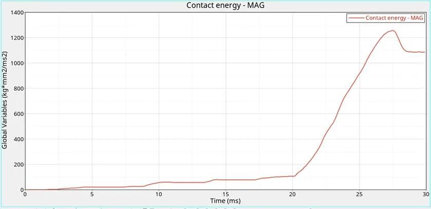
• Contact Energy:
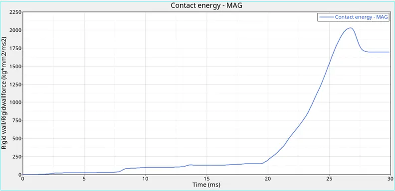
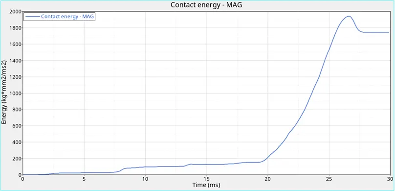
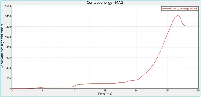
  • Contact energies are found to be much higher in the first two cases where two notches were present.
  • It is much lower when the notches are removed.
  • In all cases, the value peaks around 26 -27 ms and then becomes constant 1 ms after the peak.
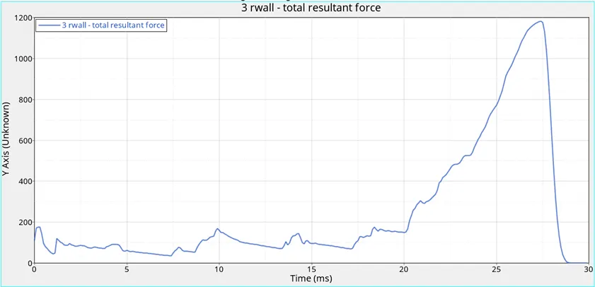
• Rigid wall forces (total resultant)
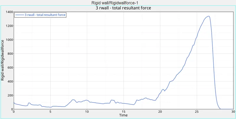
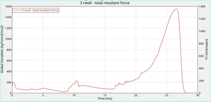
  • The Graphs are quite similar in all the cases.
  • Small peaks are observed in the initial stages (0-20 ms)
  • The largest peak occurs when the whole model gets crushed (26-27 ms).
  • Cases 5 and 6 show only one noticeable small peak before the largest peak and this might be due to the presence of only a single notch

Thus, the model that was given was meshed and the crush tube was simulated and results compared to identify the changes caused by notches and interfaces in the simulation.