Comparing the Types of Failure Shown by Different Material Cards with specific Failure Cards on a Simulation of a Rigid Sphere Crashing onto a Plate using Radioss.

Objective: To simulate the event of a rigid sphere crashing onto a flat plate as seven cases with different material and failure models for the plate and to compare them on the basis of:

1. Total number of cycles, Energy error, mass error and simulation time.
2. Animations of all the 5 and to describe the animations in brief on the basis of whether the elements are being deleted or cracked.
3. Energies and to notice any difference in the graphs plotted.
4. Results, to identify which case would represent the on-field scenario.

To document and list down the case by case result and conclusion as to why the failure happened.

Procedure:

Case 1: To simulate with both Failure Plastic strain (Eps_P_max) and fail_johnson failure card enabled.

1. Go to File -> Import Deck and select the file given.

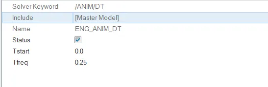
2. Set the ENG_ANIM_DT animation frequency to 0.25 as shown below, to get a smoother animation.

3. Check the Material and Failure card to check the values that are given as input.

4. The material Law used is Material Law 2 and Failure card is failure_johnson which is enabled.

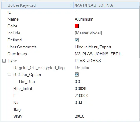
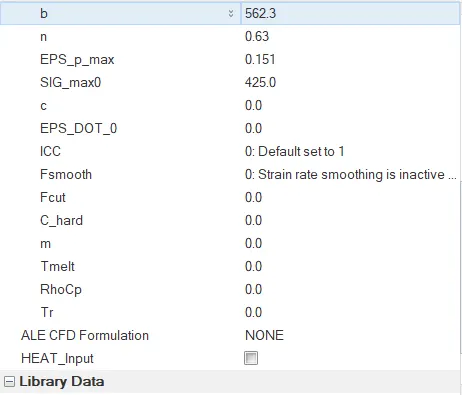
5. Save the file as Law2_epsmax_failure and run the simulation by going to Analysis -> Radioss.

6. The Hyperworks solver will show the following:

7. As we can see, the Mass and Energy Error percentage is in the allowable limits and hence we can move forward.

8. The Simulation for Von Mises Contour looks like this:

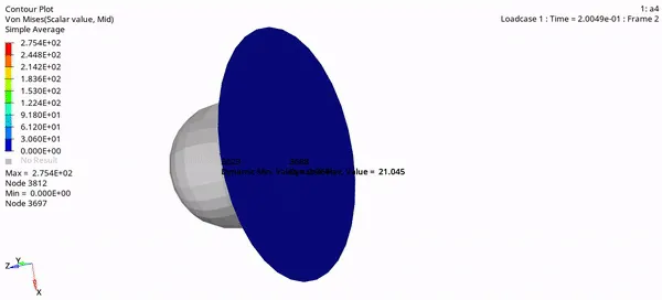
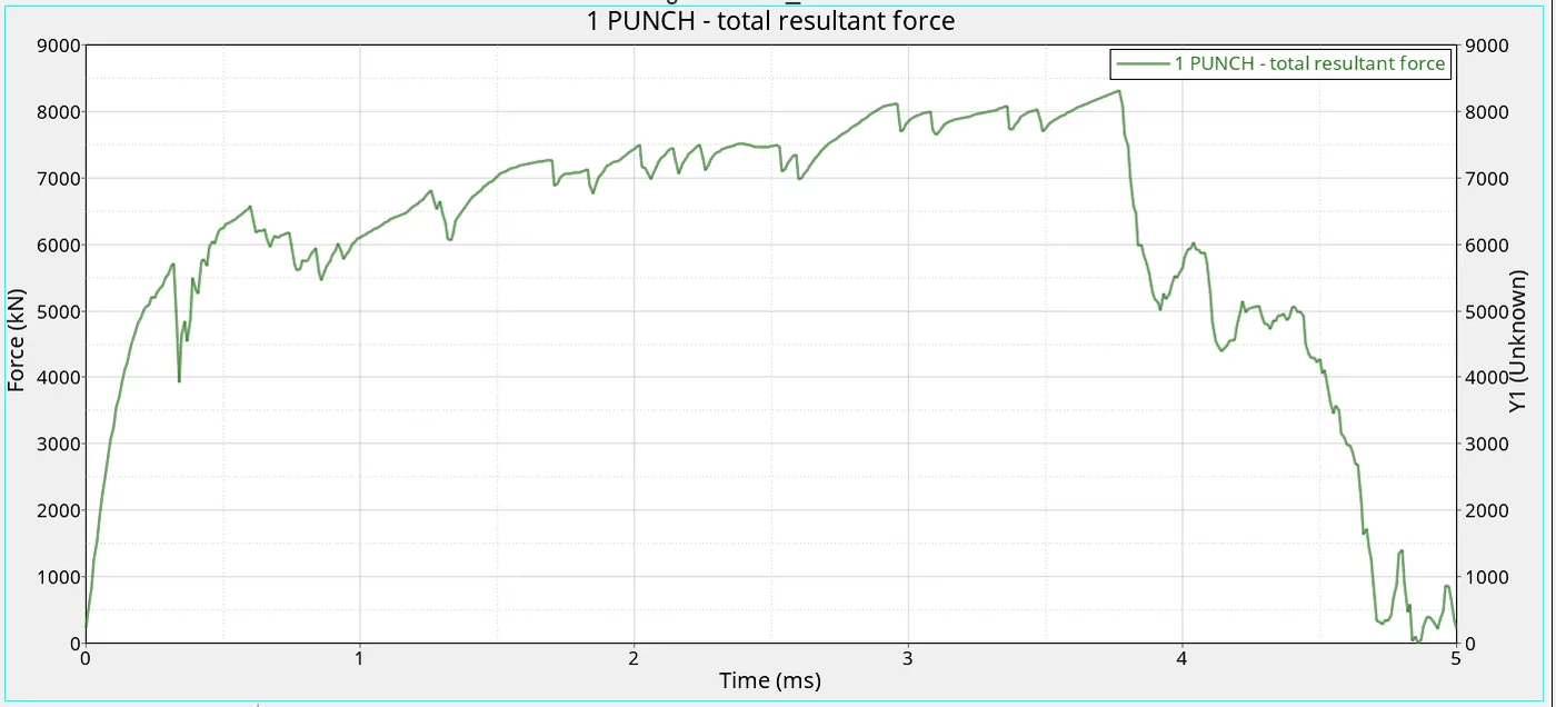
9. Plot the graph for the parameters required (Internal energy, Kinetic Energy, Hourglass energy and Total Energy)

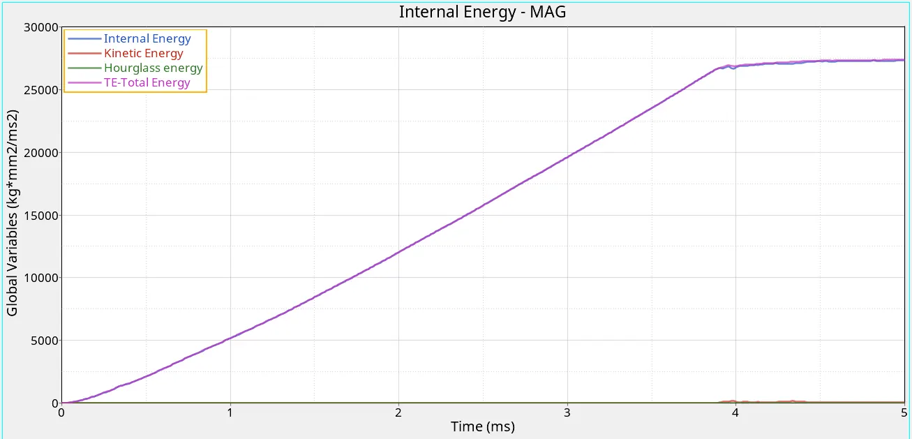
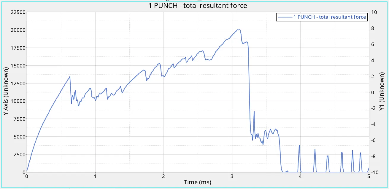
10. The Plot Resultant Normal and Tangent forces:

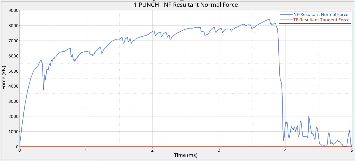
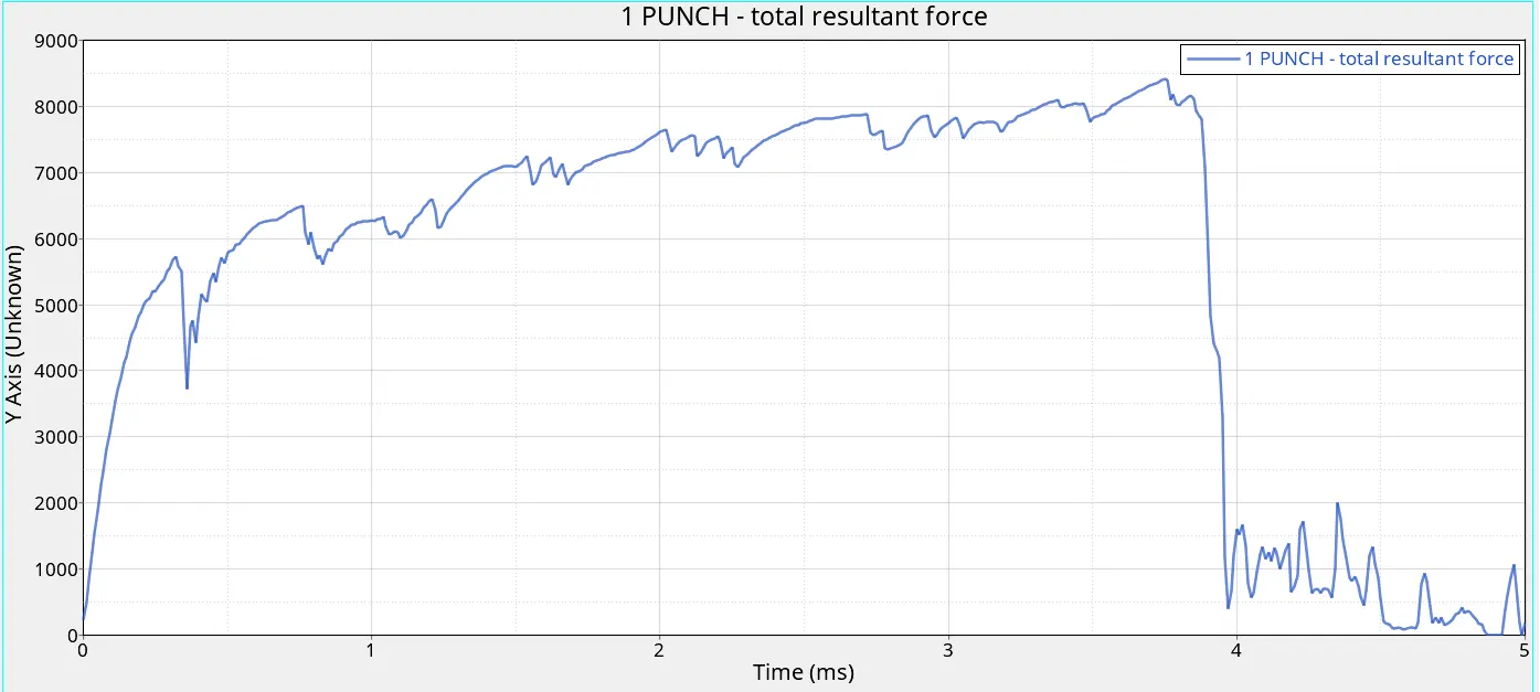
11. Since the tangent force is zero, the total force comes out to be equal to the Resultant force.

Case 2:

1. In Case 2, the steps 1 to 4 of the previous case are performed.

2. The values of failure_Johnson_1 are edited as follows:

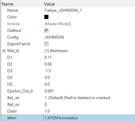
2. The simulation is run after saving the file as Law2_epsmax_crack.

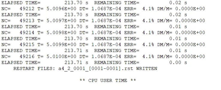
3. It is noticed that the Mass and Energy Error percentage is in the allowable limits and hence we can move forward.

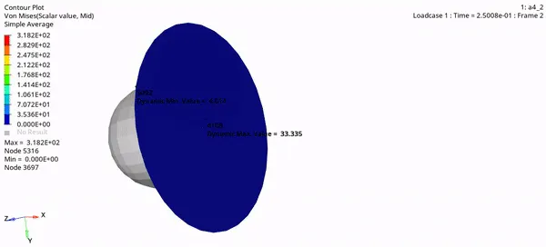
4. The Simulation for Von Mises Contour looks like this:

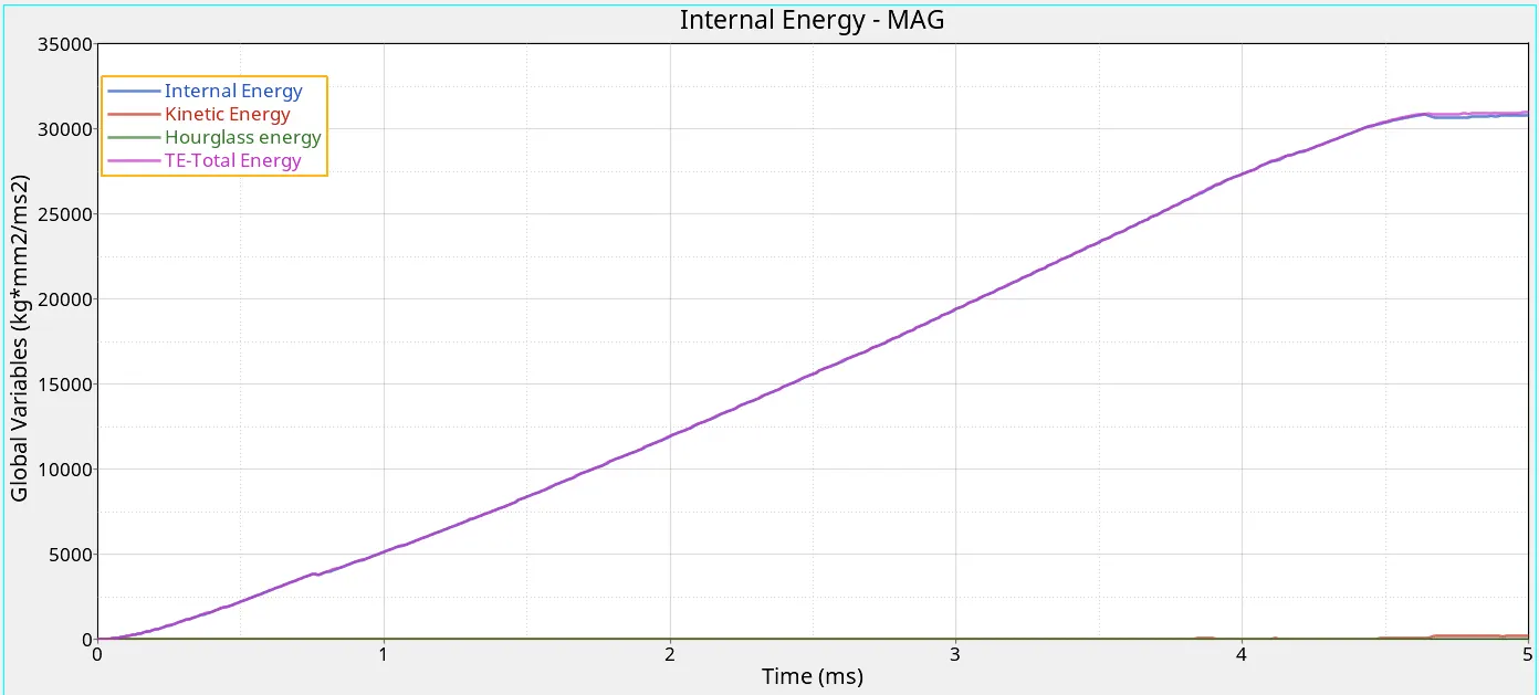
5. Plot the graph for the parameters required (Internal energy, Kinetic Energy, Hourglass energy and Total Energy)

6. The Plot Resultant Normal and Tangent forces:

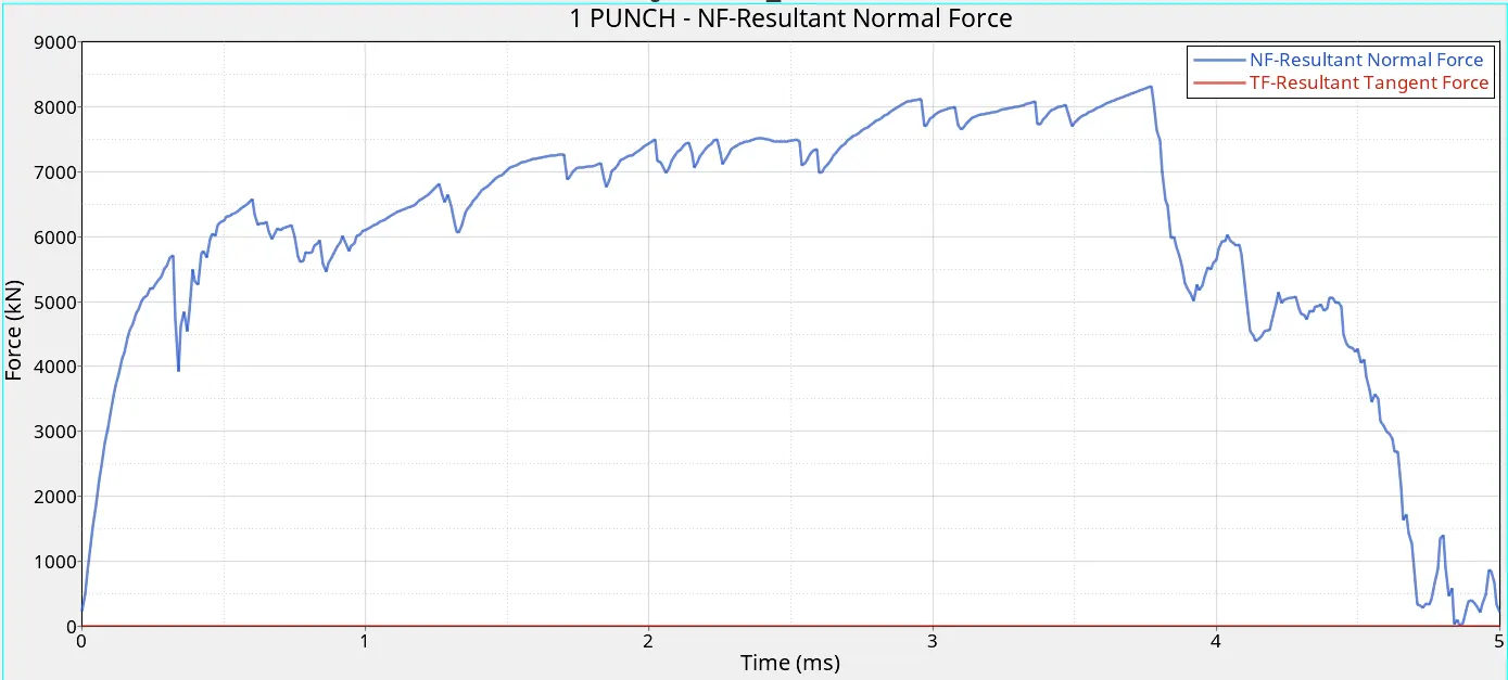
7. Since the tangent force is zero, the total force comes out to be equal to the Resultant force.

Case 3:

1. In the same file we delete the Failure Card and run the simulation to check the results.

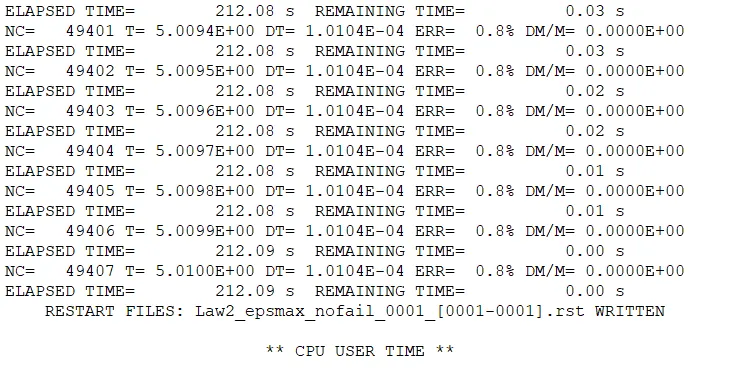
2. Save the file as Law2_epsmax_nofail.

It is noticed that the Mass and Energy Error percentage is in the allowable limits and hence we can move forward.

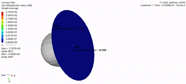
3. The Simulation for Von Mises Contour looks like this:

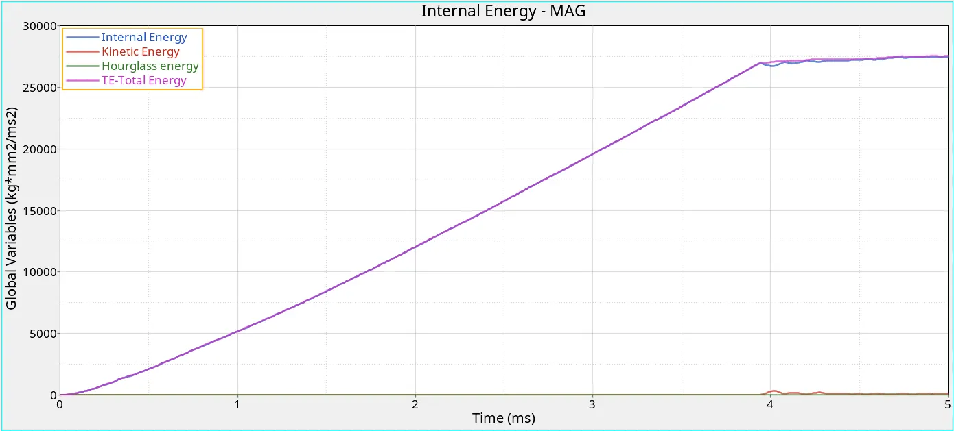
4. Plot the graph for the parameters required (Internal energy, Kinetic Energy, Hourglass energy and Total Energy)

5. The Plot Resultant Normal and Tangent forces:

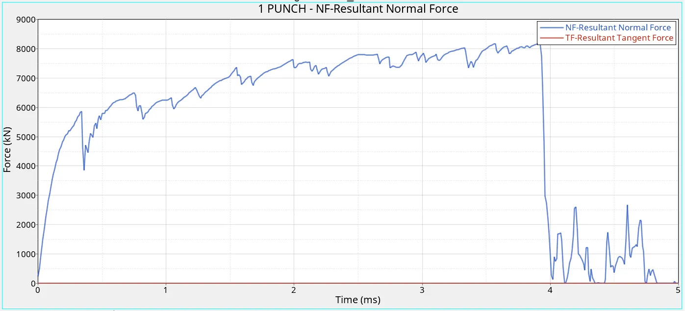
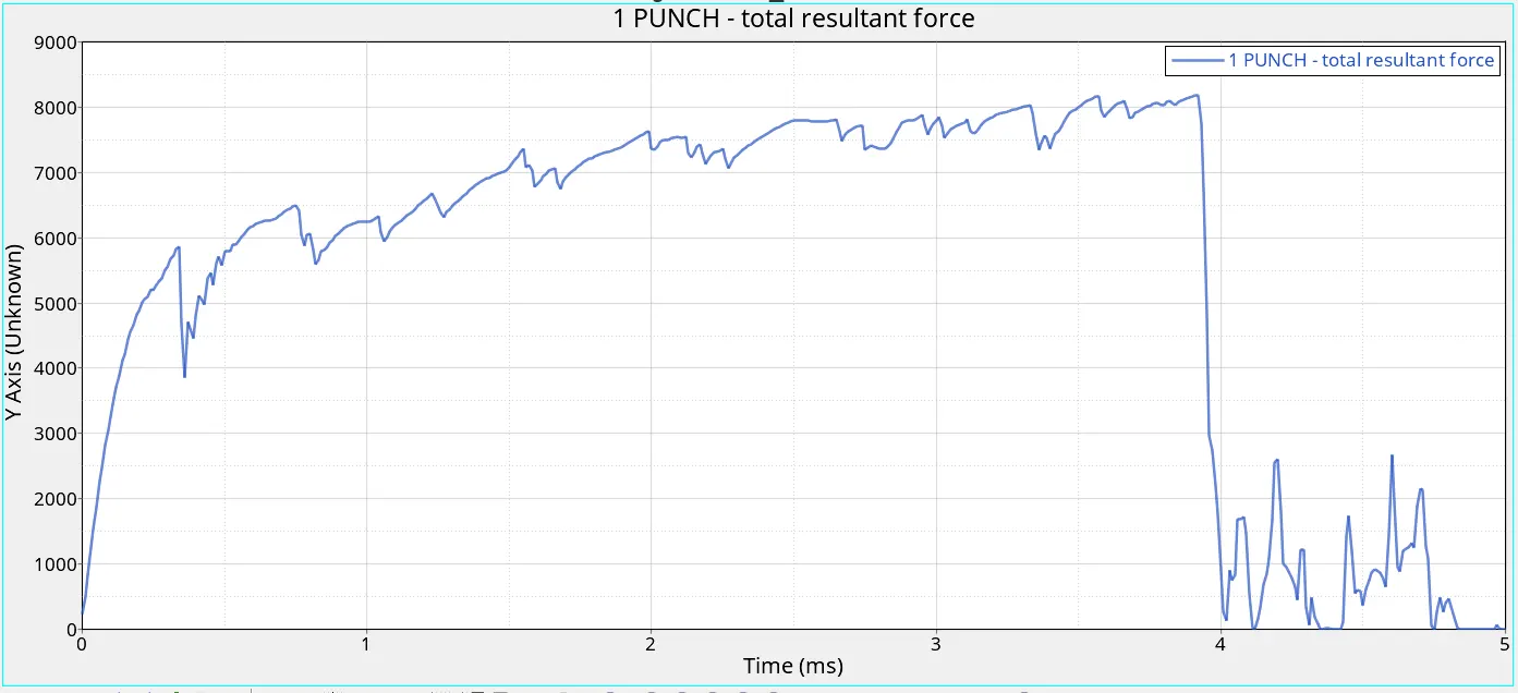
6. Since the tangent force is zero, the total force comes out to be equal to the Resultant force.

Case 4:

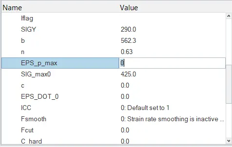
1. In the Materials Card, set the EPS_p_max value to 0 and run the simulation by following the same steps above.

2. Save the file as Law2

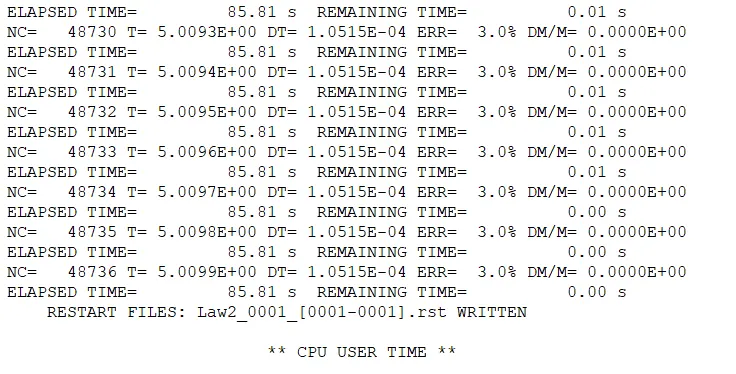
3. It is noticed that the Mass and Energy Error percentage is in the allowable limits and hence we can move forward.

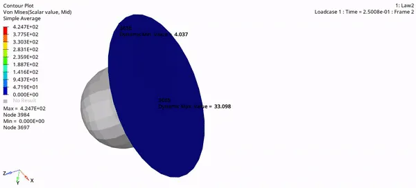
4. The Von mises stress contour of the simulation looks like this:

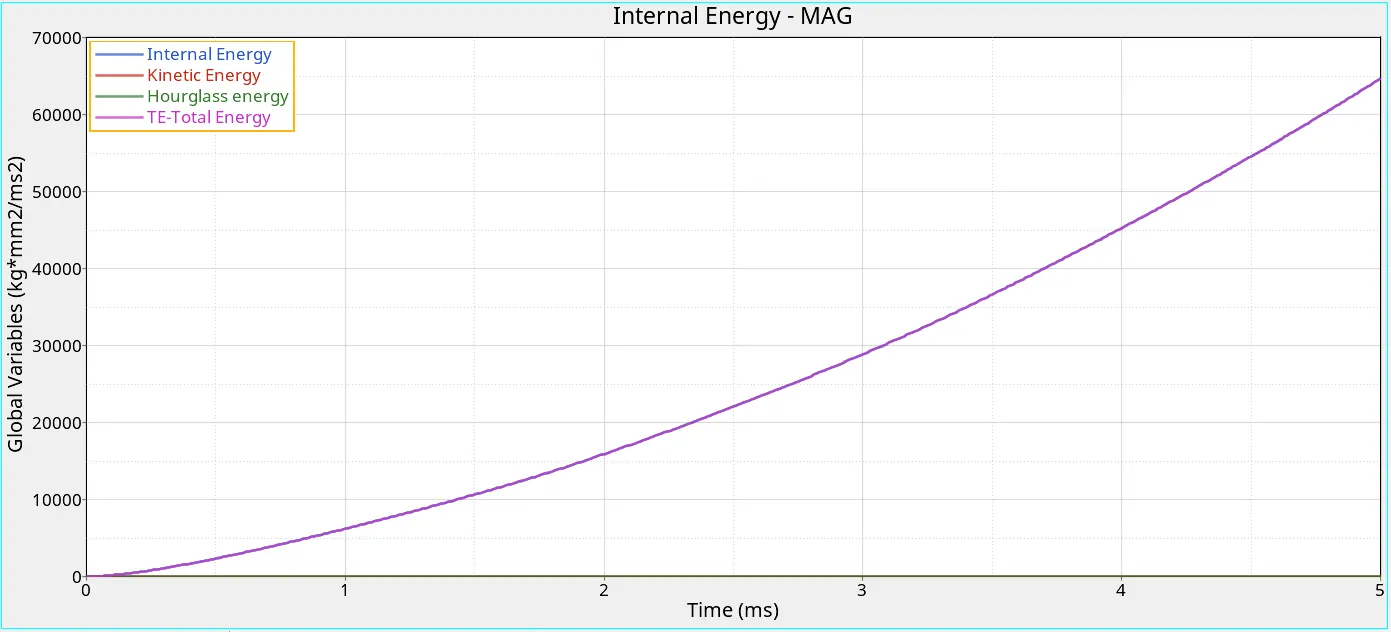
5. Plot the graph for the parameters required (Internal energy, Kinetic Energy, Hourglass energy and Total Energy)

6. The Plot Resultant Normal and Tangent forces:

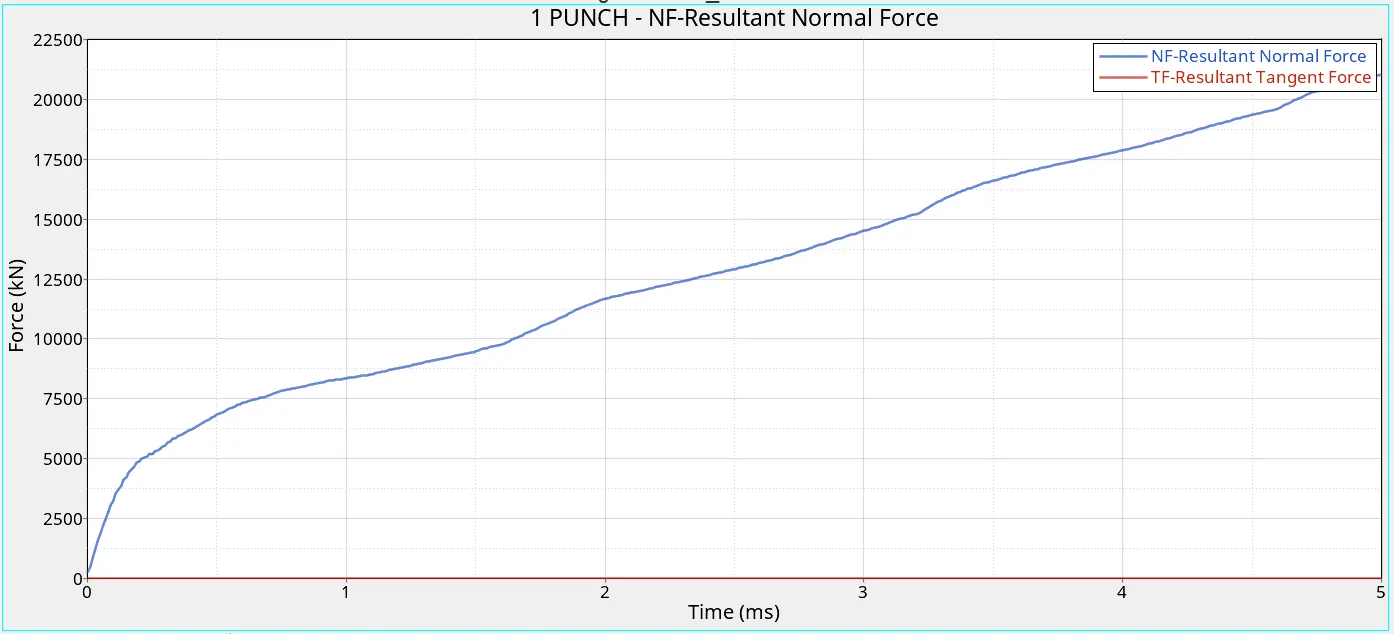
7. Since the tangent force is zero, the total force comes out to be equal to the Resultant force.

Case 5:

1. The Material Card is now changed to M1_ELAST which resembles elastic materials.

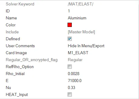
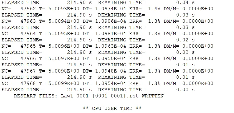
2. The file is saved as Law1 and simulated using the previus steps.

3. It is noticed that the Mass and Energy Error percentage is in the allowable limits and hence we can move forward.

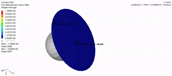
4. The Von mises stress contour of the simulation looks like this:

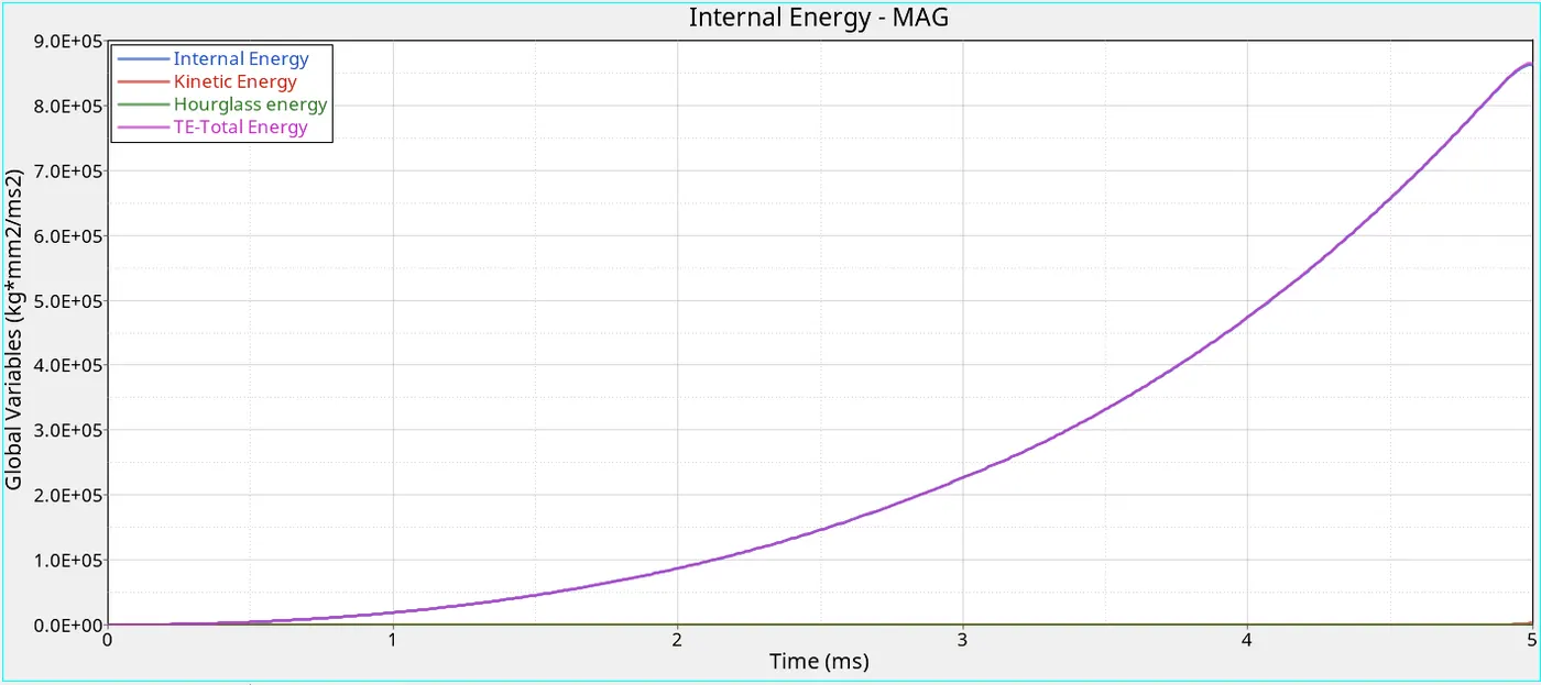
5. Plot the graph for the parameters required (Internal energy, Kinetic Energy, Hourglass energy and Total Energy)

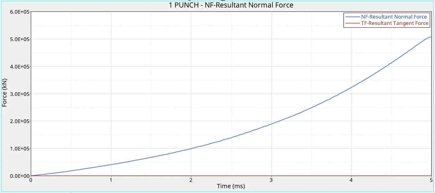
6. The Plot Resultant Normal and Tangent forces:

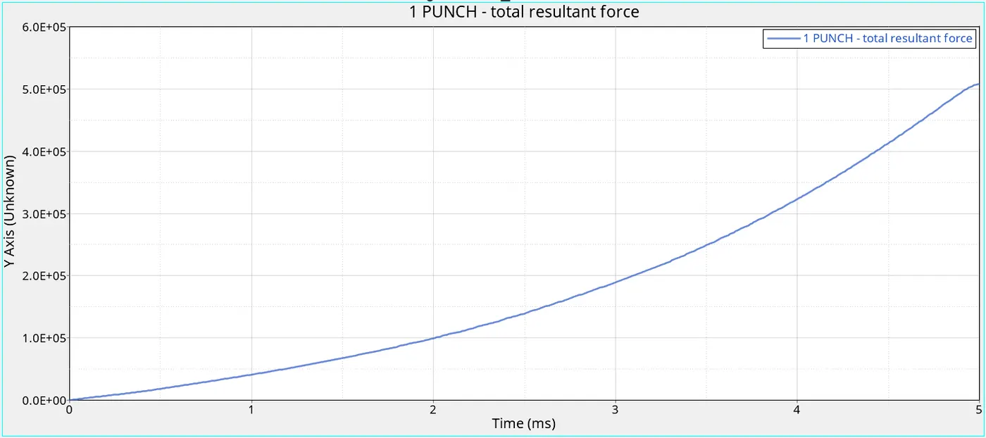
7. Since the tangent force is zero, the total force comes out to be equal to the Resultant force.

Case 6:

1. Import a new solver deck Law27_0000.rad and change the properties to recommended shell properties.

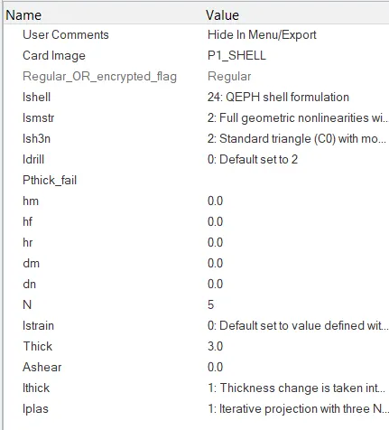
2. Run the simulation after saving the file as Law27.

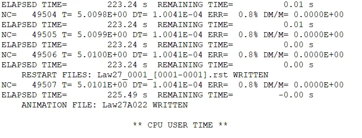
3. The errors are within the limits, so we can proceed.

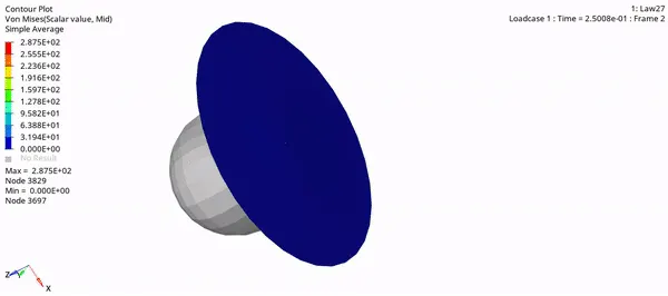
4. The Von mises contour simulation is as follows:

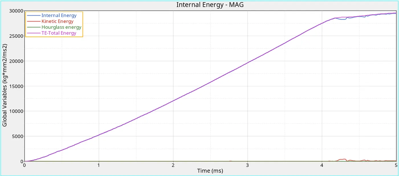
5. Plot the graph for the parameters required (Internal energy, Kinetic Energy, Hourglass energy and Total Energy)

6. The Plot Resultant Normal and Tangent forces:

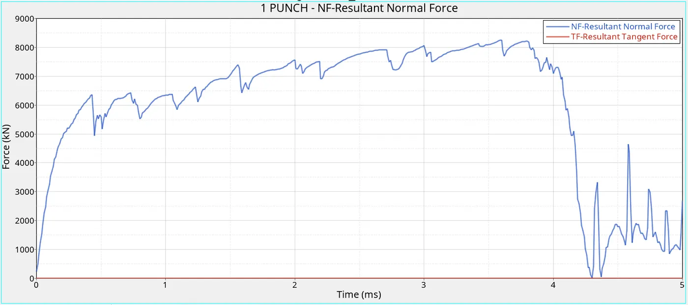
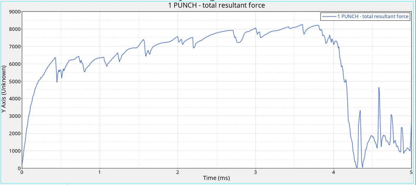
7. Since the tangent force is zero, the total force comes out to be equal to the Resultant force.

Case 7:

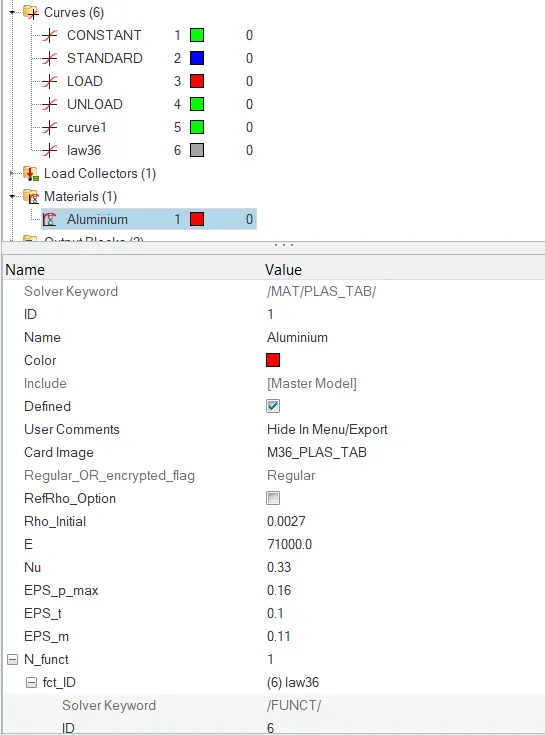
1. Change the material law to Law 36 and enter the values as shown below:

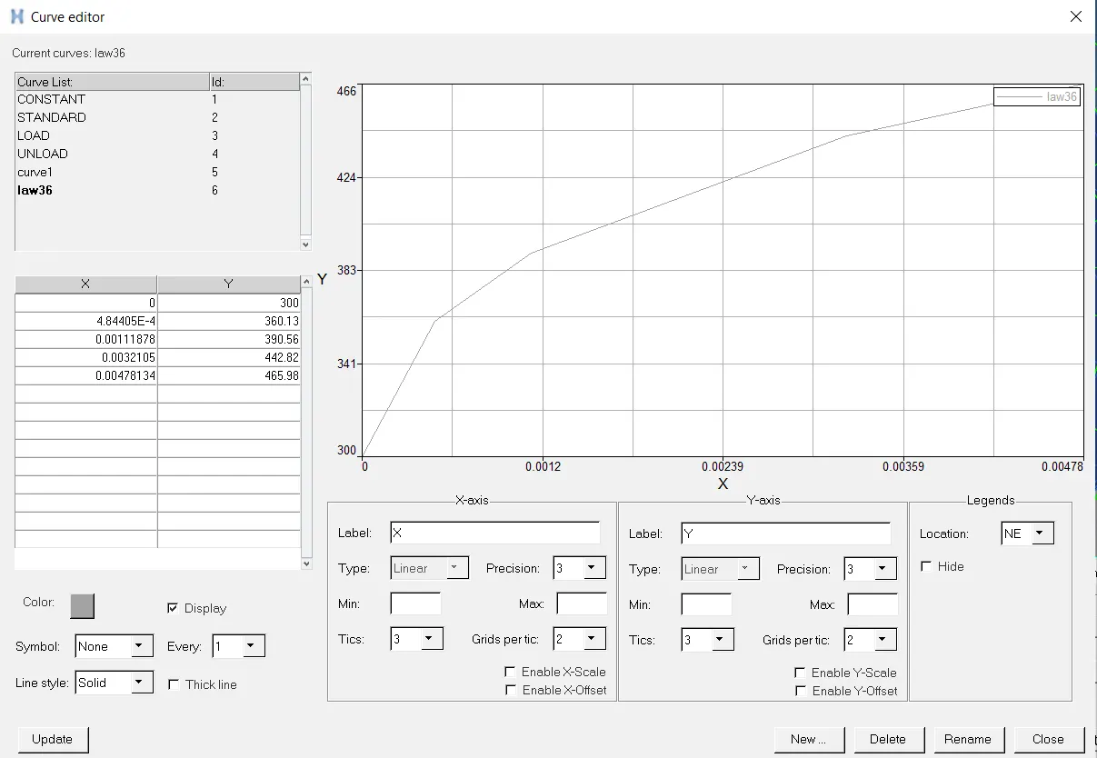
2. Create a new curve by plotting the points as shown and set that curve as the fct_ID for the material.

3. Run the simulation by following the steps mentioned above.

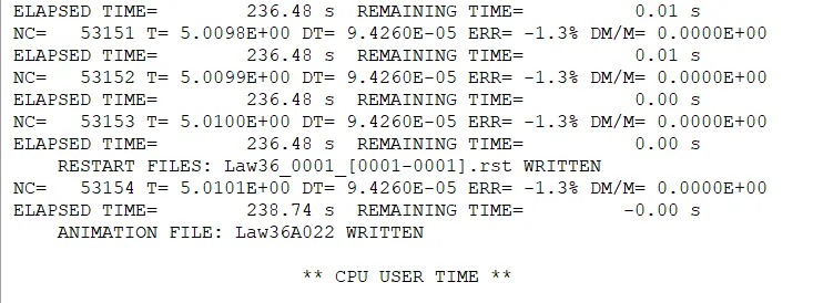
4. The errors are in the acceptable range and hence we acn proceed.

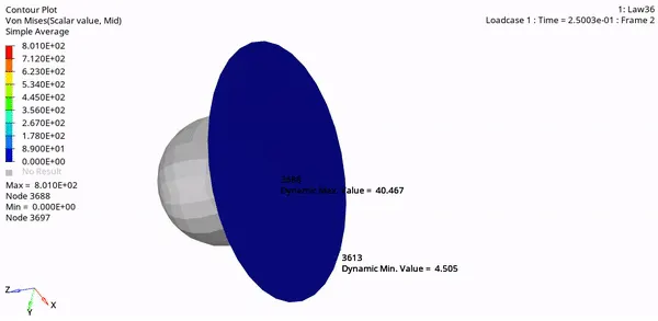
5. The Simulation for Von Mises Stress is as follows:

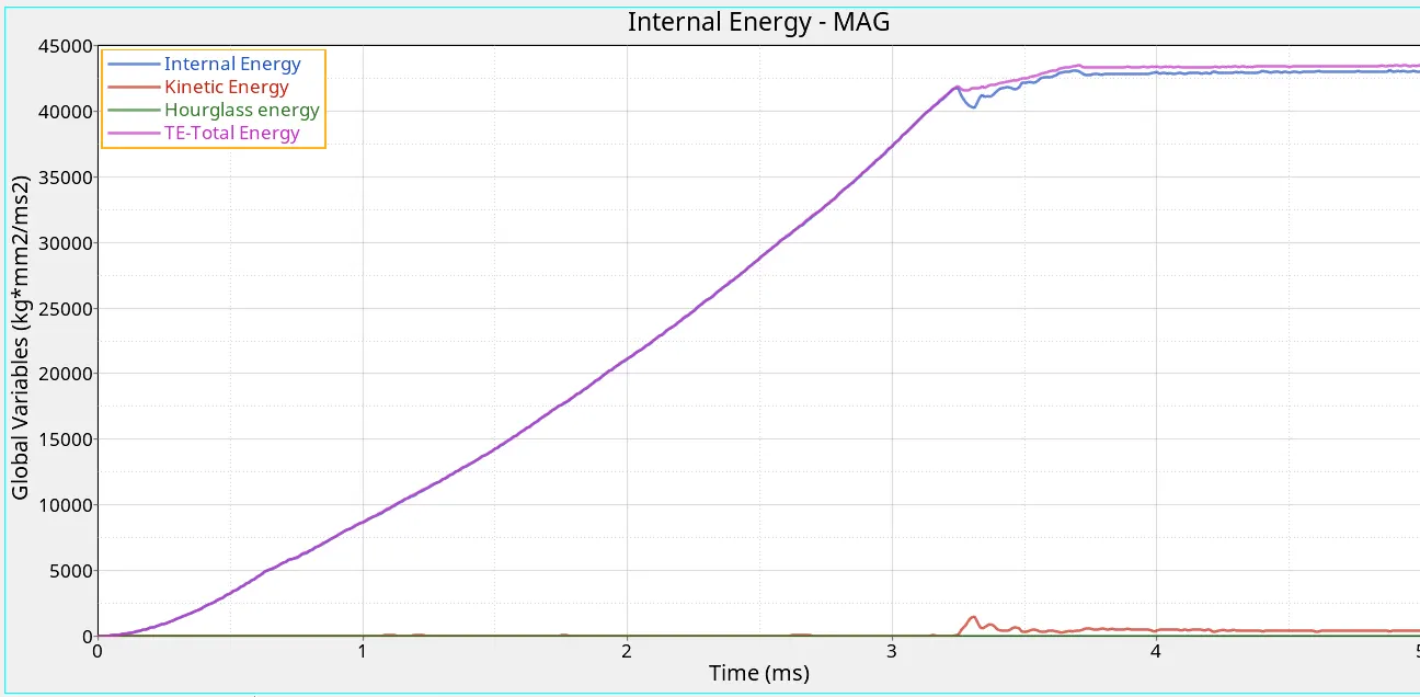
6. Plot the graph for the parameters required (Internal energy, Kinetic Energy, Hourglass energy and Total Energy)

7. The Plot Resultant Normal and Tangent forces:

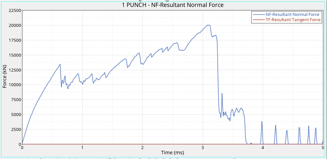
8. Since the tangent force is zero, the total force comes out to be equal to the Resultant force.

Results and Comparison:

Comparson 1:

Let us first compare a few parameters such as Number of Cycles, Energy and Mass Error and Simulation time.

Case	No. of Cycles	Energy Error %	Mass Error	Total Simulation time (s)
1	49380	0.8	0	224.20
2	49217	4.1	0	229.30
3	49408	0.8	0	220.76
4	48737	3	0	90.11
5	47969	1.3	0	218.93
6	49508	0.8	0	232.70
7	53155	-1.3	0	240.50

Conclusion 1:

• We notice that the number of cycles is the lowest in the case 5 where we used Material Law 1 and highest in case 7 where we used Material law 36.
• Energy Error is lowest positive in Case 1,3,6 and lowest negative in case 7.
• Mass Error is zero in all the cases.
• The total Simulation time is the highest in case 7 and lowest in case 4.

Comparison 2: Animation

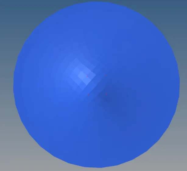
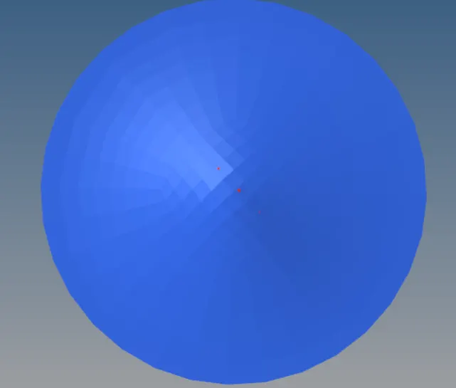
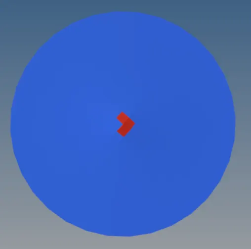
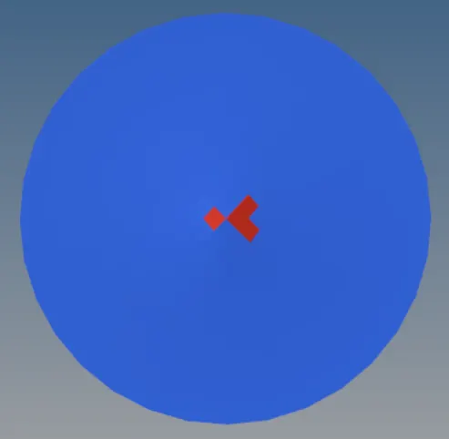
Shown below are the animation and types of failure (deletion or crack) for all the 7 cases.

Case	Animation	Screenshot of initial failure	Type of failure
1			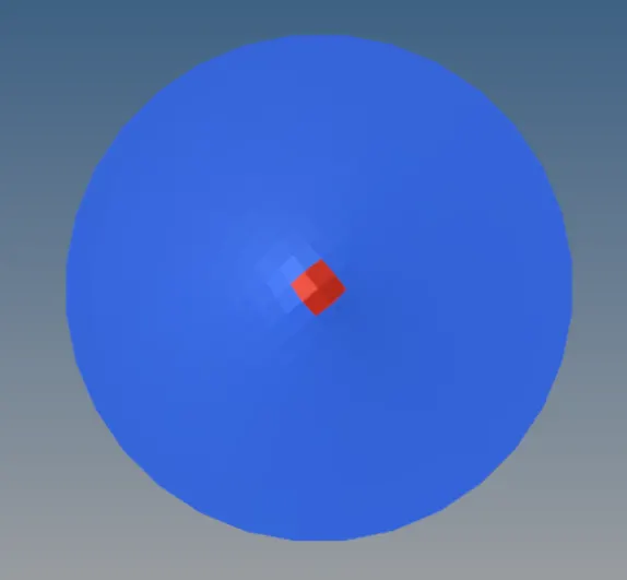Deletion
2			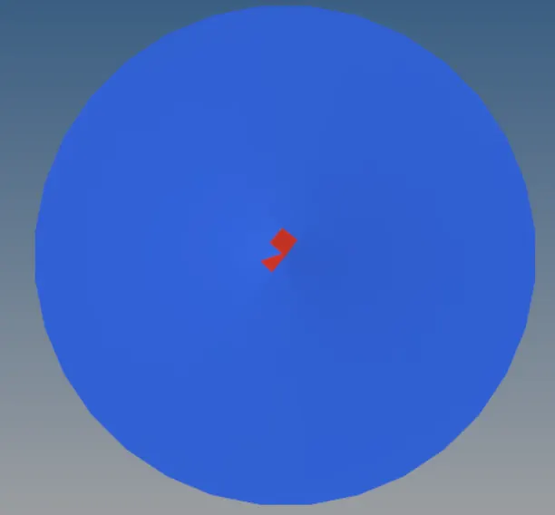Crack
3			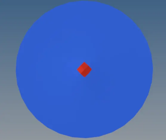Deletion
4			NA
5			NA
6			Deletion
7			Deletion

Comparison 3: Energies

Case	Energy Plot	Remarks
1		A linear increase in both TE and IE till ~ 4 ms. A constant value of TE and IE is observed after ~ 4 ms A dip in IE and Increase in KE at ~ 4ms Total Energy is almost equal to IE. Kinetic Energy is very small as compared to the other values. HGE remains zero throughout Max energy ~ 27500 MJ
2		A linear increase in both TE and IE till ~ 4.5 ms. A constant value of TE and IE is observed after ~ 4.5 ms A dip in IE and increase in KE at ~ 4.5ms Total Energy is almost equal to IE. Kinetic Energy is very small as compared to the other values. HGE remains zero throughout Max energy ~ 32000 MJ
3		A linear increase in both TE and IE till ~ 4 ms. A constant value of TE and IE is observed after ~ 4 ms A dip in IE and Increase in KE at ~ 4ms Total Energy is almost equal to IE. Kinetic Energy is very small as compared to the other values. HGE remains zero throughout Max energy ~ 27500 MJ
4		A non-linear increase in TE and IE through the simulation HE remains zero. Max energy ~ 65000 MJ
5		An exponential increase in TE and IE through the simulation HE remains zero. Max energy ~ 850000 MJ
6		A linear increase in both TE and IE till ~ 4.2 ms. A slowly increasing value of TE and IE is observed after ~ 4.2 ms A dip in IE and Increase in KE at ~ 4.2 ms Total Energy is almost equal to IE. Kinetic Energy is very small as compared to the other values. HGE remains zero throughout Max energy ~ 29000 MJ
7		A non linear increase in both TE and IE till ~ 3.2 ms. A slowly increasing value of TE and IE is observed after ~ 3.2 ms till 3.8 ms and then a constant value till the end of the simulation A dip in IE and Increase in KE at ~ 3.2 ms Total Energy is almost equal to IE. Kinetic Energy is very small as compared to the other values. HGE remains zero throughout Max energy ~ 43000 MJ

Conclusions based on Observations:

• Choosing the Material Law plays a vital importance to capture the material of the model properly and get accurate results for the type of simulation.
• Random material cards will show results but it will not be accurate and relatable to a real life scenario.
• The Material Laws and their uses:
  • Law 1: Used for purely elastic materials in the elastic range. To model this, we require the Poisson's ratio and Young's Modulus. It represents a linear relationship between Stress and Strain.
  • Law 2: Behaves as linear elastic when equivalent stress is lower than Yield stress and for higher values of stress, the material behaves as a plastic. Better failure can be captured by using the Failure Johnson card.
  • Law27 : Used for Brittle materials
  • Law 36: In this, Elastic-Plastic behaviour of isotropic materials is modeled using user defined functions. The Stress - Strain curve is modeled using E and Poisson's ratio. The Hardening behaviour of the material is a function of plastic strain for a given strain rate.
• The type of material card that needs to be used depends on the type of material of the plate that we are trying to simulate.
• Case 4 and 5 (Law2 and Law1) show infinite strain failure limits and are hence not recommended.
• Case 6 (Law27)can be used in the case of a brittle material.
• Case 1 and 7(Law2 with failure card + failure plastic strain enabled and Law36) show promising results, however, case 7 (Law36) gives us more control by allowing us to use stain curve data which was obtained by experimental methods.