Side Pole Crash Analysis on a Dodge Neon BIW Model using Radioss.

Objective:

To perform a side pole crash analysis on a Dodge Neon BIW Model.

We are required to perform the following operations:

• Check unit system and either follow [Mg mm s] or [Kg mm ms].
• Create appropriate interface with friction 0.2 and recommended parameters.
• Make sure to clear all penetration and intersections.
• Create a rigid wall with friction 0.1.
• Compare the model weight with the reference model and use added masses to reach target weight 700kg while getting CG about the required range.
• Set an Initial velocity of 35mph.
• Use model checker to ensure good quality.
• Set the Timestep as 0.5 to 0.1 microseconds.
• Run the simulation for 80ms.

Output requests:

• Sectional force in the cross member.
• Intrusion at B pillar,hinge pillar and fuel tank region.Provide recommendation on what can help to reduce Fuel tank intrusion.
• Peak velocity of inner node of the door.

Procedure:

1. Open the Hyperworks window and import the solver deck that is given.

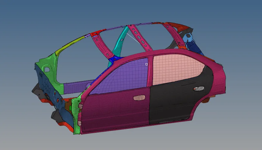
2. The model will look as follows:

3. We begin by checking the unit system.

4. Open the BEGIN_CARD and check the units used as shown below.

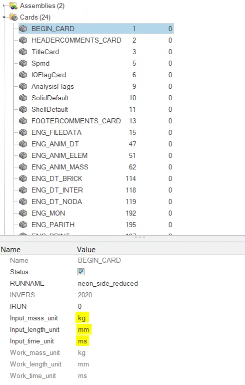
5. Thus we can conclude that we follow kg, mm, ms units.

6. Next we create the Rigid wall/ Pole.

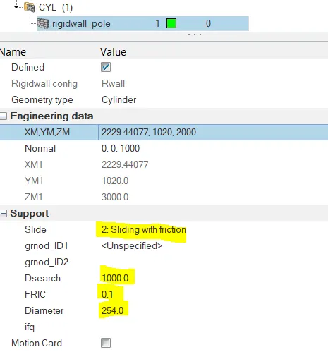
7. Right click in the solver tab -> Create -> RWall -> Cylinder.

8. Set the parameters as highlighted below:

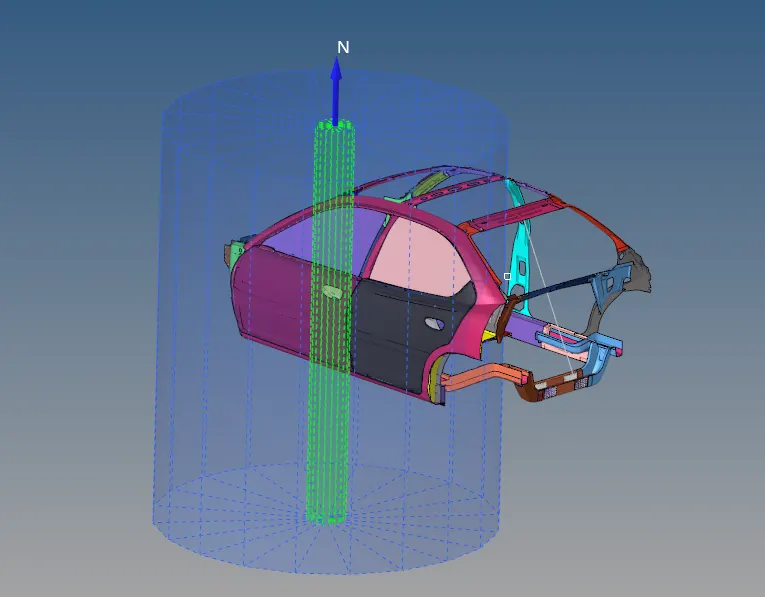
9. The rigid wall and model created will look as shown below:

10. Next, let us set the simulation time.

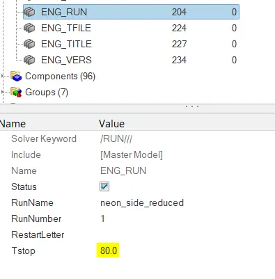
11. Go to the ENG_RUN file and set Tstop value as 80.

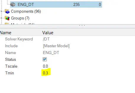
12. Next we set the timestep by going to the ENG_DT card and set Tmin as 0.3 as shown below:

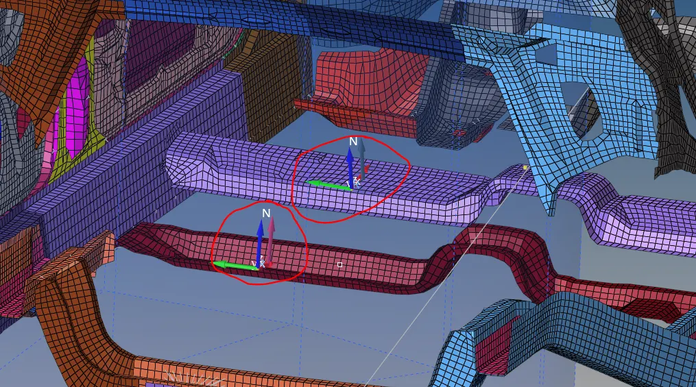
13. Next we check for Penetrations by going to tools -> Penetration check and perform the check as shown below:

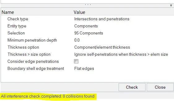
14. Since no penetrations were found, we can continue.

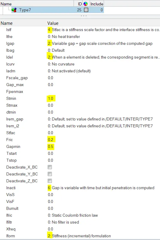
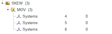
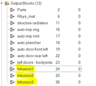
15. Let us create a new Type7 Interface with recommended properties as shown below.

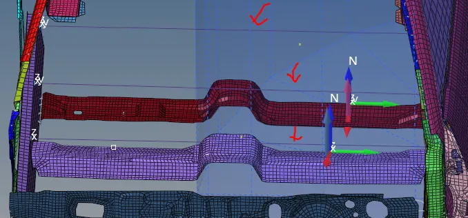
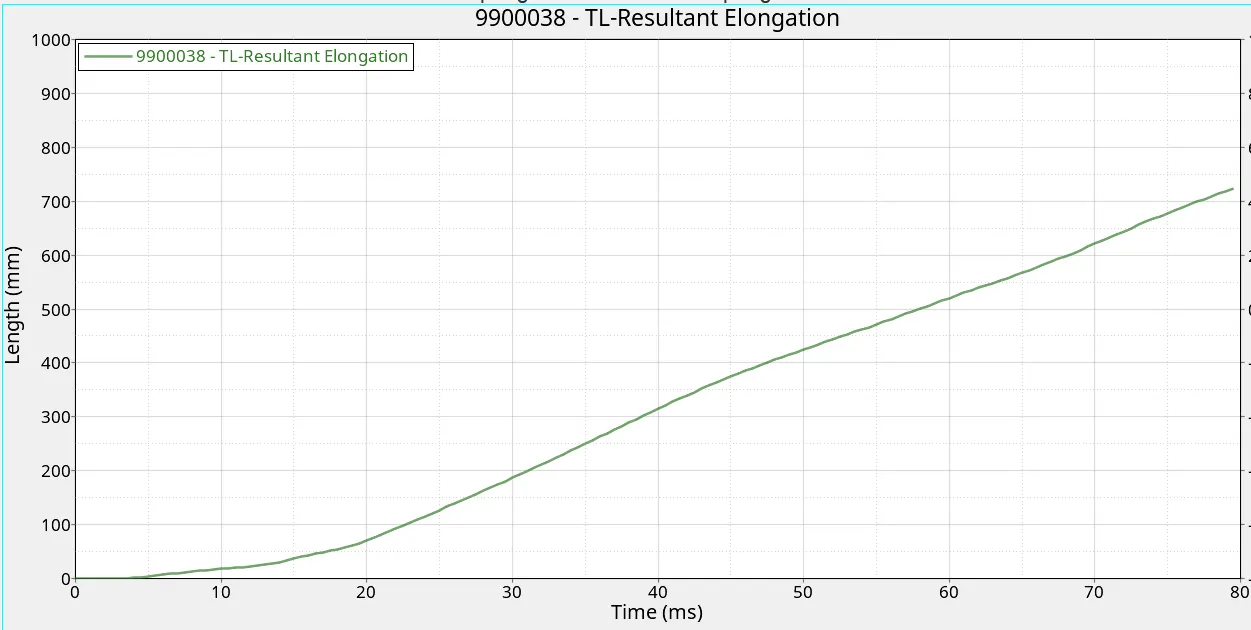
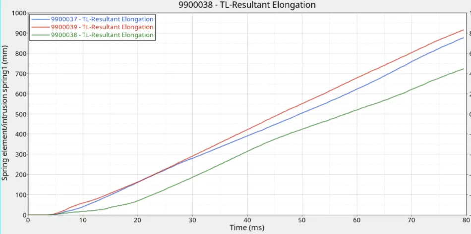
16. Set the master and slave as self and continue.

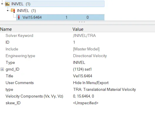
17. Set the INIVEL as shown below.

18. Convert 35 mph to mm/ms to get 15.6464 mm/ms.

19 This value is applied along the positive y axis.

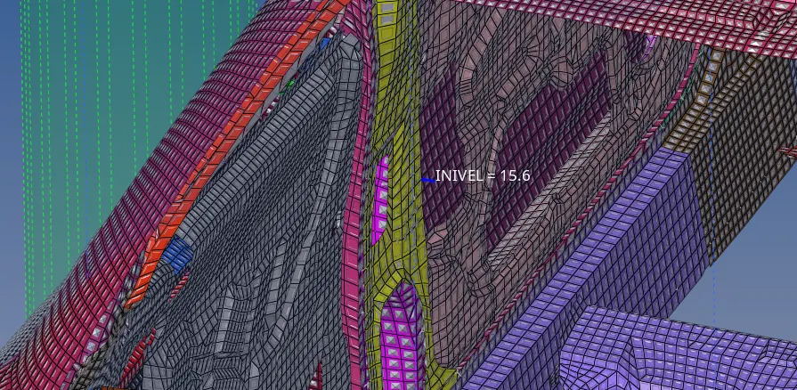
20. The vector notation will show the direction and magnitude of the applied velocity for us to check.

21. The next step is to set the COG and mass correctly:

22. For this we use the ADMAS card and select the nodes to apply the masses on.

23. Old COG:

x - 2420.6088301742557

y - 248.4562368888605

z - 588.9372731394064

24. New COG:

x- 2610.10516189549

y - 61.39266659567736

z - 342.36004156072096

25. The old and new COGs are shown below:

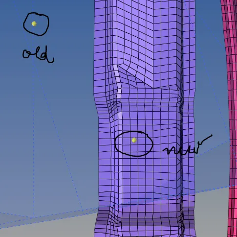
26. The total mass has also reached the target value of 700kg as required.

27. Next we set up the Output requests such that we get the required values to plot graphs.

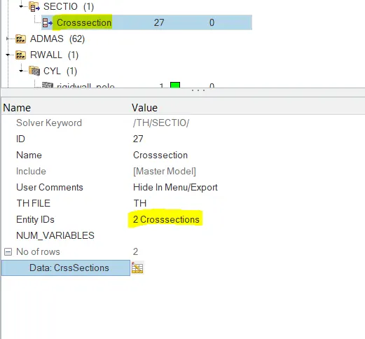
28. We start by creating Cross Sections. Create a new section by Right clicking on the Solver tab -> Create -> SECT.

29. We create a FRAME if necessary to define the section better and select the nodes and elements as required.

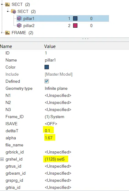
30. The cross-members, after specifying the cross section looks as follows:

31. Similarly we set up the intrusions on the B pillar,hinge pillar and fuel tank region.

32. For this, we set up skews that align in the same line as the nodes mentioned above and select the corresponding skew to measure the intrusion onto the dashboard.

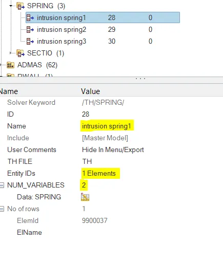
33. Another way to measure this is by creating Spring elements as shown below and measuring how much the element is deformed.

34. Both these methods are accepted. We have tried following both these methods:

Spring elements:

35. We now request for the Peak velocity as an output parameter of the inner node of the door as shown below:

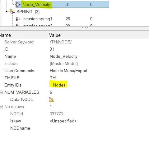
35. Now we set the parameters in the output block so that we get a the required outputs.

36. Output Parameters for spring intrusions:

37. Output Parameters for Cross-sections:

38. We then check the Model using the Model Checker. Tools -> Model Checker -> Radioss Block.

39. After rectifying any errors that may have crept in, we can run the simulation.

40. Go to Analysis -> Radioss, set the options to -nt 4 and click Radioss.

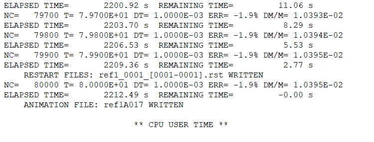
41. The Mass and energy error are within the acceptable range and hence we can continue.

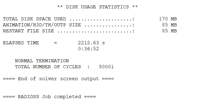
42. The simulation ran for 80001 cycles and took around 37 mins to simulate.

Results:

1. We open the animation files to view the results as shown below:

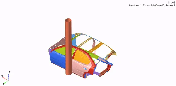
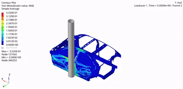
2. Von Mises Contour:

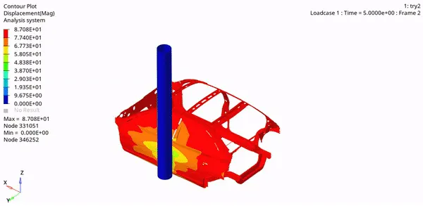
3. Displacement Contour:

4. We open the T01 file to plot the required graphs as shown below:

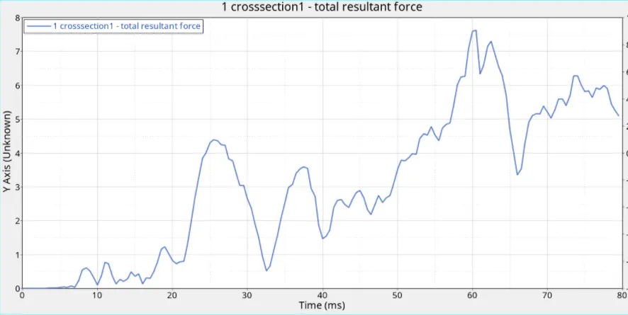
Sectional force in cross member 1:

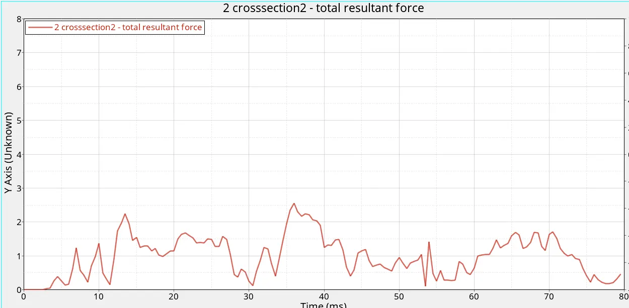
Sectional force in cross member 2:

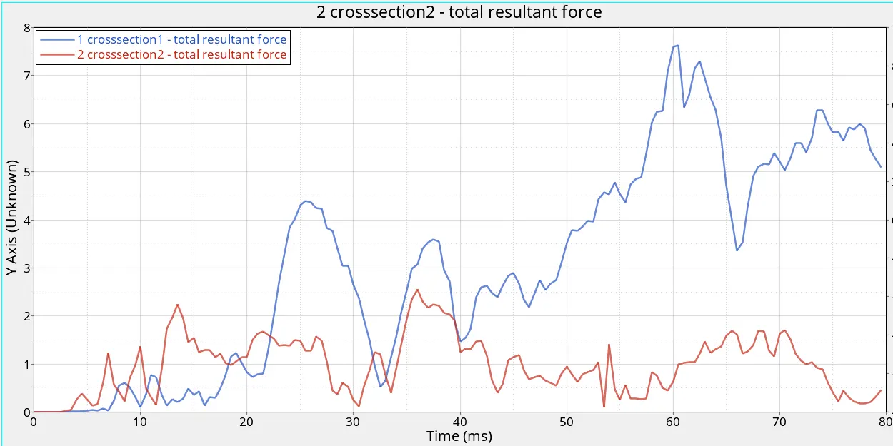
Sectional force in cross member 1 and 2 plotted together:

Conclusions:

• The values of forces are much higher on cross section1 as compared to cross section 2.
• The force peaks at ~7.5kN for cross section1
• The force peaks at ~2.5kN for cross section2
• This difference can be accounted for by the different cross sections of the cross members.
• Another reason for the dissimilarity of forces might be due to the positioning of the members to the impacted pole.

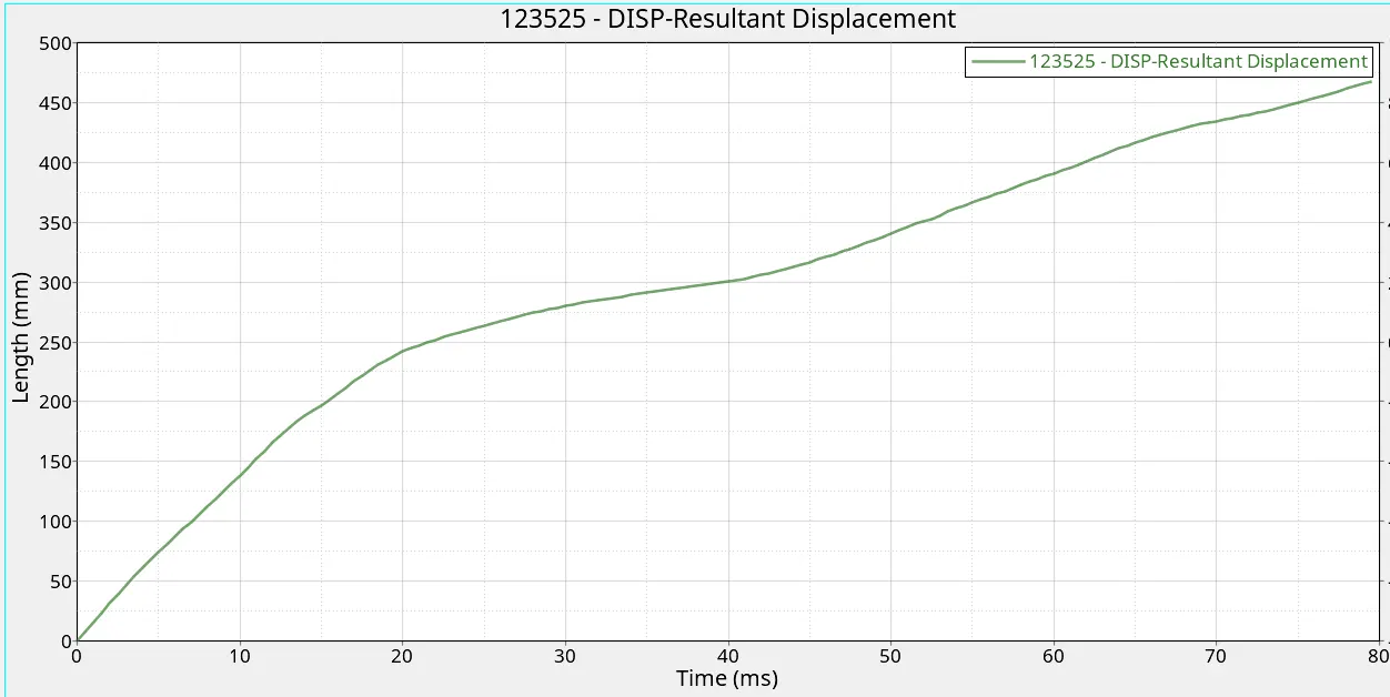
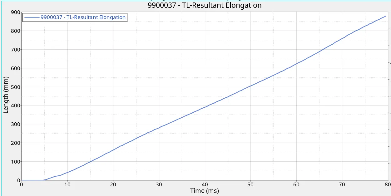
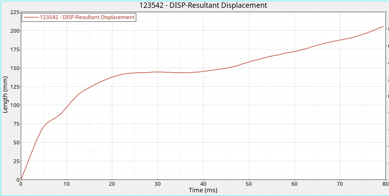
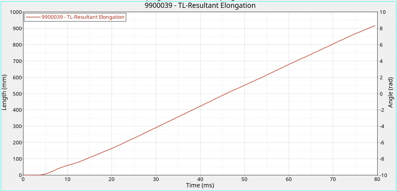
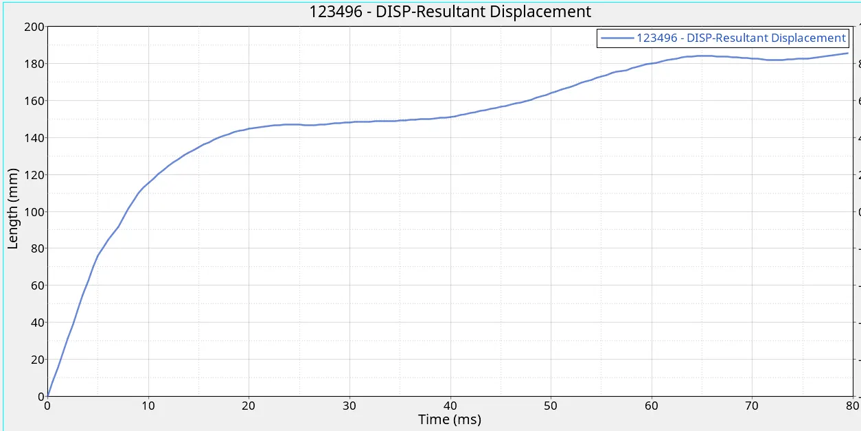
Now let us do a comparison to find intrusions using both the methods discussed:

Sno	Intrusion	Spring
1	Intrusion : 1329 - 475 = 854 mm	Max resultant elongation: 880mm
2	Intrusion : (1330 - 210) = 1120mm	Max resultant elongation: 910 mm
3	Intrusion : 1327 - 190 = 1137 mm	Max resultant elongation: 710mm

Conclusions:

• Since Spring deformation provide more accurate results, we can conclude that those values are more true.
• The highest intrusion is at the centre nodes and this is due to the fact that that region is closest to the impact region.
• The Fuel tank region experiences an intrusion of 880mm.
• The side impact crash is very dangerous because this is the impact is extremely close to the passengers.
• Fuel tank intrusions can be reduced by:
  • Providing an anti-intrusion bar to absorb the kinetic energy.
  • Adding a possible additional cross member to share the load.
  • Using better material selection.
  • Providing better padding and a design that can absorb the energies more efficiently.

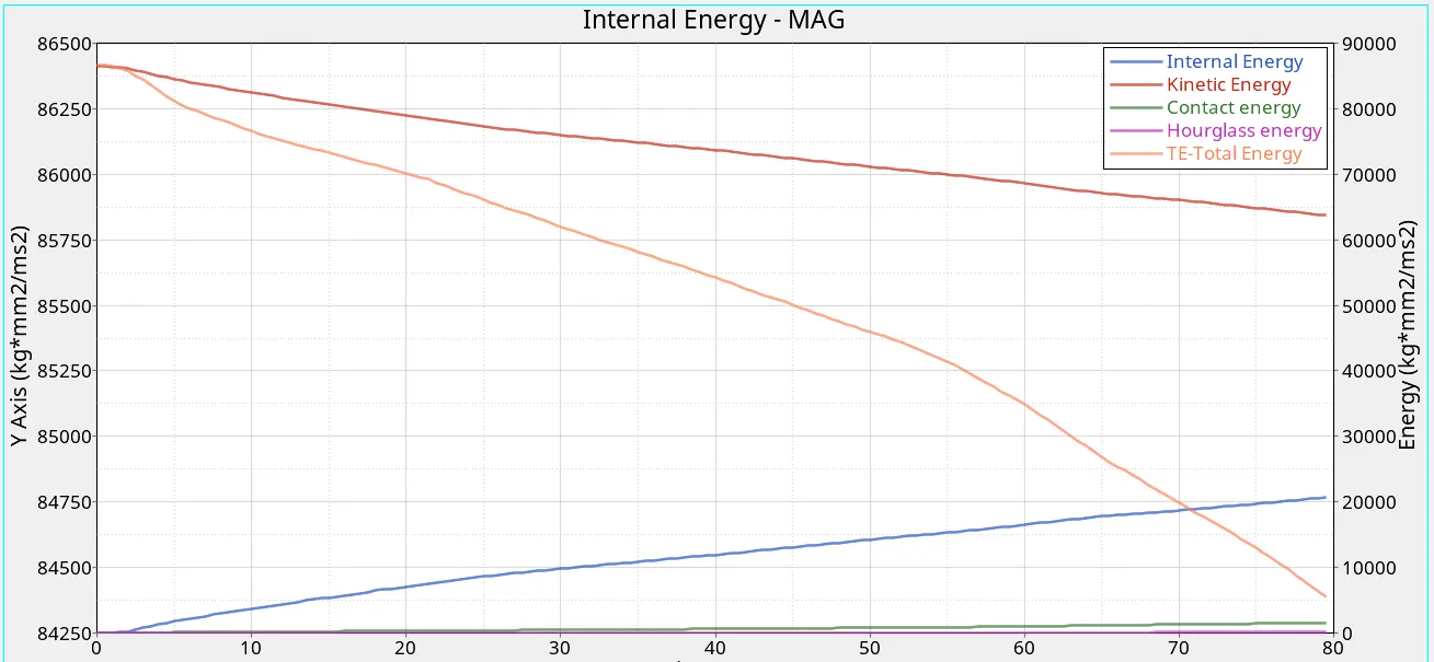
Plot for Energies:

Conclusions:

• Total energy shows a steady decrease from ~86300 kg*mm2/ms2 to ~5000 kg*mm2/ms2
• Kinetic energy shows a steady decrease from ~86300 kg*mm2/ms2 to ~5000 kg*mm2/ms2
• Internal energy shows a steady increase from ~0 kg*mm2/ms2 to ~20000 kg*mm2/ms2
• Contact energy is almost minimal throughout.
• Hourglass energy is zero throughout.

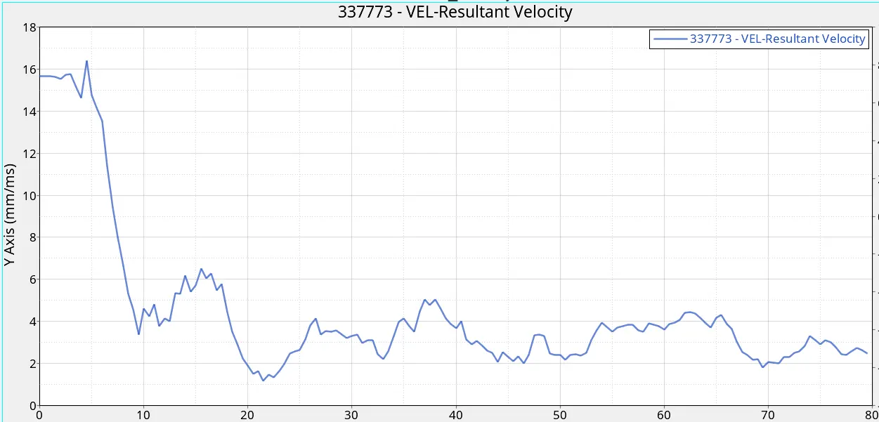
Plot for Peak Velocity:

Conclusion:

• Peak velocity of the was reached at ~5ms with a magnitude of ~16.2 mm/ms.
• This can be connected to the initial impact.
• A sudden decrease is then observed.
• This is followed by a varying velocity in the range of ~1 to 6 mm/ms.

Thus, the model was simulated for a side pole crash test and the results were discussed.