Week 9 - FVM Literature Review

The Finite Volume Method (FVM):

It is a popular numerical technique used primarily for the simulation of fluid flow and heat transfer. It is widely used in the field of computational fluid dynamics (CFD). Here's a simplified explanation of how it works:

1. Domain Discretization: The physical domain of the problem is divided into a finite number of small, control volumes (CVs) or cells. This grid can be structured, unstructured, or hybrid.
2. Integral Form of Governing Equations: Instead of using the differential form of the governing equations (as in FDM), FVM uses their integral form. The equations representing the physical conservation laws (mass, momentum, energy, etc.) are integrated over each control volume.
3. Flux Calculation: The net flux of the conserved quantity through the control volume boundary is computed. This involves calculating the amount of the quantity entering and leaving the CV.
4. Volume Averaging: The conserved variables are calculated and stored at the centroids of the CVs, and their values are assumed to be representative of the entire CV.
5. Discretization: The integral equations for each control volume are discretized to create algebraic equations. The discretization translates the fluxes across the CV surfaces into algebraic terms involving the neighboring CV values.
6. Solution of Algebraic Equations: The set of algebraic equations for all CVs is solved iteratively to obtain the distribution of the conserved quantities across the domain.

In the context of FVM, interpolation schemes are methods used to estimate the values of physical quantities at the CV faces from the cell-centered values. Since the conservation equations are solved at the CV faces, accurate estimation of these face values is critical for the fidelity of the simulation.

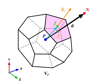
• The volume of the control volume is denoted as V and is centered around point P, which serves as the centroid.
• The vector from centroid P to centroid N is referred to as d.
• Knowledge about all neighboring control volumes is available.
• Control volume faces are labeled f, representing the face center.
• The point where the vector d intersects a face is denoted as f.
• The face area vector points outward from the control volume, is positioned at the face centroid, is normal to the face, and has a magnitude equal to the area of the face.
• The vector from centroid P to face center f is termed Pf.

Differential Form of FDM:

Major differences between the Finite Difference Method (FDM) and the Finite Volume Method (FVM):

1. Discretization Approach:
   FDM: Discretizes the differential equations directly by approximating derivatives at discrete points.
   FVM: Integrates the differential equations over control volumes, focusing on the fluxes crossing the boundaries of these volumes.
2. Conservation:
   FDM: May not strictly enforce conservation laws at the discrete level.
   FVM: By design, it enforces the conservation of quantities (e.g., mass, momentum, energy) across control volumes.
3. Grid Flexibility:
   FDM: Typically uses structured grids, which limits flexibility in handling complex geometries.
   FVM: Can be applied to structured and unstructured grids, allowing it to handle complex geometries more easily.
4. Accuracy and Stability:
   FDM: Accuracy is directly related to the stencil and can be less stable for advection-dominated problems.
   FVM: Uses a median-dual approach to provide stability, especially with the use of flux limiters and interpolation schemes.
5. Boundary Conditions:
   FDM: Boundary conditions are applied at discrete points, which can sometimes be challenging for irregular boundaries.
   FVM: Boundary conditions are applied over the faces of control volumes, which can more naturally handle irregular boundaries.

Interpolation schemes used in FVM method are as follows:

• Upwind Interpolation Scheme. (UDS)
• Central Differencing Approximation. (CDS)
• Quadratic Upwind Differencing Scheme. (QUICK)
• Hybrid Interpolation Scheme. (CDS & UDS)
• Total variation Diminishing Scheme. (TVD)

1. The upwind interpolation scheme: It is primarily employed for convection-dominated problems. This scheme is essentially analogous to utilizing the forward or backward difference methods, depending on the direction of flow. The determination of variable values in the interpolation process is contingent upon the velocity direction at a given point. Accordingly, the node upwind or upstream from the specified node is utilized, aligning with the scheme's namesake.

For approximating the value of the variable 'f' at the east face of the control volume, the expression for the Upwind Interpolation (UDS) is as follows:

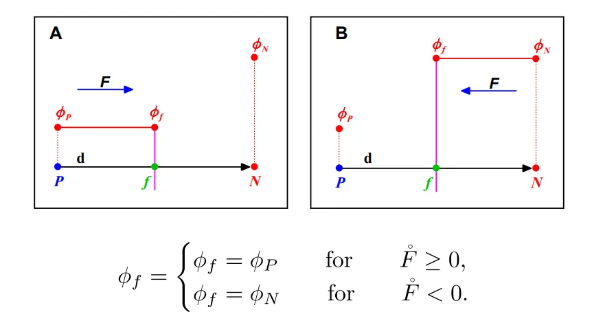
One distinctive advantage of the upwind interpolation is its unconditional satisfaction of the boundedness criterion. Regardless of the velocity values and grid spacing, the solution always remains bounded. This characteristic makes upwind interpolation a reliable choice that inherently avoids generating oscillatory solutions.

This type of interpolation scheme is known as upwind differencing and it is first order accurate.This scheme is bounded (non-oscillatory) and diffusive.

Advantages:

The Upwind Differencing Scheme (UDS) possesses the distinctive advantage of being the sole approximation method that unconditionally satisfies the boundedness criterion. This unconditional satisfaction holds true regardless of the velocity and grid spacing, ensuring that oscillatory solutions are never generated.

Disadvantages:

Despite its merits, UDS comes with certain drawbacks. Notably, it introduces numerical diffusion, and this diffusive effect is accentuated, especially in multi-dimensional scenarios when the flow is oblique to the grid. The consequence of this numerical diffusion is the smearing out of peaks or rapid variations in the variables. Another limitation is that UDS is only first-order accurate, necessitating the use of very fine grids to achieve accurate solutions.

2. Central Differencing Approximation (CDS):

The Central Differencing Scheme (CDS) is a widely used numerical method in computational simulations, particularly in the realms of fluid dynamics and heat transfer. Employed for approximating spatial derivatives, CDS relies on linear interpolation between neighboring points to estimate the gradient of a variable within a discretized domain. The formula for CDS involves computing the difference in variable values at points ahead and behind a given location, divided by twice the grid spacing. This simple yet effective approach renders CDS second-order accurate, providing a reasonable balance between computational efficiency and accuracy in capturing spatial variations. However, caution is warranted, as CDS may exhibit oscillatory behavior, especially in the presence of sharp gradients or discontinuities. Despite this limitation, CDS remains widely adopted due to its simplicity and versatility, serving as a foundational element in numerical methods and facilitating the understanding of more advanced schemes.

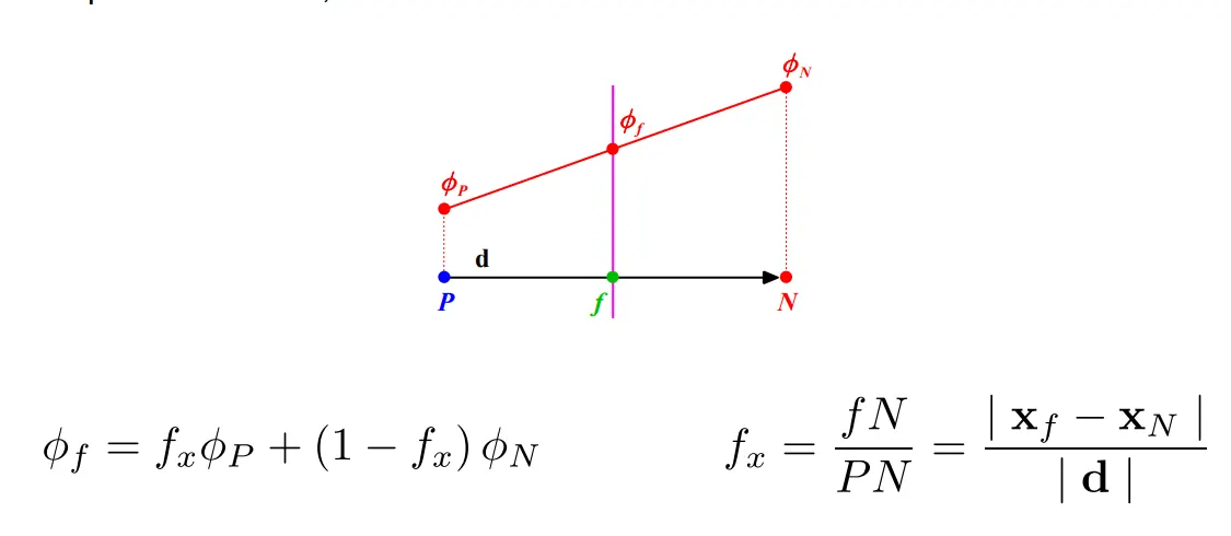
This type of interpolation scheme is known as linear interpolation or central differencing and it is second order accurate. However, it may generate oscillatory solutions (unbounded solutions).

3.Quadratic Upwind Interpolation:

Quadratic Upwind Interpolation for Convective Kinematics (QUICK) is used to interpolate values at the faces of control volumes in computational fluid dynamics simulations. The QUICK interpolation scheme involves a quadratic expression to estimate the variable of interest based on values at three neighboring grid points. The general equation for QUICK interpolation can be expressed as follows:

`f_e = f_P + 1/4 * (3 * (f_N - f_P) - (f_{NN} - f_P))`

In this equation:

`f_e` is the estimated value at the face of the control volume.

`f_P` is the value at the control volume centroid.

`f_N` is the value at the nearest downstream grid point.

`f_{NN}` is the value at the second nearest downstream grid point.

QUICK interpolation uses a weighted average of the values at the centroid, nearest downstream point, and second nearest downstream point to provide a more accurate estimate, particularly in the context of convective flows.

4. Hybrid Interpolation Scheme:

A Hybrid Interpolation Scheme in CFD is a computational strategy that integrates multiple interpolation methods to accurately estimate fluid properties at locations between known grid points. This method aims to leverage the strengths of different interpolation techniques, adapting to the fluid flow's intricacies and ensuring accurate representation in regions with sparse or irregularly distributed data.

Associated Equations:

The equations associated with a Hybrid Interpolation Scheme in CFD depend on the specific interpolation methods employed. Let's consider a combination of linear and polynomial interpolation for illustration:

Linear interpolation between grid points `(x_1,u_1)` and `(x_2,u_2)`.

• Linear Interpolation in CFD (for simplicity):
  `u_{linear}(x) = u₁ + ((x - x₁) * (u₂ - u₁)) / ||x₂ - x₁||`

Linear interpolation between grid points (�1,�1) and (�2,�2): �linear(�)=�1+(�−�1)⋅(�2−�1)∥�2−�1

• Polynomial Interpolation in CFD (for accuracy):
  Polynomial interpolation of degree n using (n+1) neighboring data points: Hybrid Interpolation in CFD:
  `u_{poly}(x) = Σ_{i=0}^n a_i (x - x₁)^i`

• Hybrid interpolation combining linear and polynomial methods:
  `u_{hybrid}(x) = w * u_{linear}(x) + (1 - w) * u_{poly}(x)`
  
  Here, w is a weighting factor that determines the influence of each interpolation method. The choice of w can be adjusted based on the flow characteristics and grid distribution to optimize accuracy and computational efficiency in the CFD simulation.This Hybrid Interpolation Scheme enhances the robustness of CFD simulations, allowing for accurate predictions of fluid properties in complex flow scenarios where a single interpolation method might fall short.

5. Total variation Diminishing Scheme:

The Total Variation Diminishing (TVD) scheme is a numerical method commonly employed in computational fluid dynamics to solve hyperbolic partial differential equations while preserving the total variation of the solution. The key characteristic of TVD schemes is their ability to prevent the creation of new oscillations in the numerical solution, particularly around discontinuities. Here's a brief overview with necessary equations:

`Q_i^{n+1} = Q_i^n - ((Δt) / (Δx)) * (F_{i+1/2} - F_{i-1/2}) + ((Δt) / (Δx)) * Φ(r_i) * (Φ(r_i) * F_{i+1/2} - F_{i-1/2})`

where:

`Q_i^n`is the solution at grid point i and time step n.

`F_{i+1/2}` is the numerical flux at the cell interface between i and i+1.

`Δt` is the time step, and `Δx` is the grid spacing.

`Φ(r_i)` is the limiter function based on the local slope ratio `r_i`.

The limiter function ensures that the scheme is TVD, preventing excessive overshooting or undershooting.

• The TVD scheme is designed to maintain the Total Variation (TV) of the solution at each time step, ensuring that the numerical solution remains bounded and does not introduce spurious oscillations. TV is a measure of the spatial variation of the solution.
• At each computational step, the TVD scheme employs a limiter function to adjust the solution in regions of strong gradients or discontinuities, limiting the introduction of new extrema.

FLUX LIMITERS:

Flux limiters, on the other hand, are techniques used to combine high-resolution (accurate but can produce oscillations) with low-resolution (stable but diffusive) schemes to capture sharp gradients without introducing non-physical oscillations. They are particularly important in convection-dominated flows where high-order schemes may introduce spurious oscillations.

In the realm of convective fluid flow simulations, the challenges of low-order schemes, marked by stability but dissipative characteristics around points of discontinuity or shocks, and the instability and oscillations associated with higher-order schemes, necessitate the adoption of flux limiters. These limiters play a crucial role in fine-tuning both higher and lower order schemes to achieve higher-order accuracy in the smooth regions of the flow, while maintaining first-order accuracy in the vicinity of shocks and discontinuities. The Total Variation Diminishing (TVD) criteria guide the implementation of flux limiters, ensuring that the additional convective flux, initially introduced to enhance the scheme's order, is constrained within specified limits. The flux limiter function, denoted as ϕ(r), acts as a key component in this process. The limiter function is expressed in terms of the ratio of successive gradients on the solution mesh (rᵢ), where ϕ(r) is constrained to be greater than or equal to zero. The limiter function dictates the behavior of the flux, with ϕ(r) equal to zero yielding a low-resolution scheme with sharp gradients, while ϕ(r) greater than zero corresponds to a high-resolution scheme with positive gradients. The mathematical representation of fluxes in 1D equations involves the flux limiter function adjusting the low and high-resolution fluxes to strike the desired balance between accuracy and stability. The selection of specific flux limiters is a critical aspect, involving a trial-and-error method as no universal limiter is found to work optimally for all scenarios. In summary, flux limiters emerge as indispensable tools in achieving highly accurate and oscillation-free results in convective fluid flow simulations, ensuring the balance between stability and accuracy.

It is imperative to note that flux limiters are also referred to as slope limiters because they both have the same mathematical form, and both have the effect of limiting the solution gradient near shocks or discontinuities.

`F(u_(i+1/2)) = f^(low)(i+1/2) - ϕ(r_i)(f^(low)(i+1/2)-f^(high)(i+1/2))`

`F(u_(i-1/2)) = f^(low)(i-1/2)- ϕ(r_i-1)(f^(low)(i-1/2)-f^(high)(i-1/2))`

Here, `f^(low)`=Low precision flux (1st order precise)

`f^(high)`= High precision flux (Highest order precision)

`ϕ(r)` = Flux limiter function and `r = (u_i-u_(i-1))/(u_(i+1)-u_i)`

Using the 1D linear heat conduction equation as an example:

FVM would involve integrating the heat conduction equation over each control volume. The resulting equations would relate the heat fluxes entering and exiting the CV to the rate of temperature change within the CV. Interpolation would be necessary to estimate the temperature at the CV boundaries (where the heat fluxes are calculated), and flux limiters could be used to ensure the numerical stability of the solution, particularly when dealing with sharp temperature gradients.

Finite Volume Method (FVM) Explanation:

In FVM, the domain is discretized into control volumes (CVs), and the conservation equation is integrated over each control volume. This process involves calculating the heat fluxes entering and exiting the control volume, relating them to the rate of temperature change within the CV.

Heat Conduction Equation:

`(partial T )/ (partial t )= alpha * (partial^2 T) / (partial x^2)`

FVM Discretization:

The heat conduction equation is discretized using FVM by integrating over a control volume Δx at position `x_i`:

`rho * Cp * V_i * ((dT_i)/dt) = alpha * (T_{i+1} - T_i) - alpha * (T_i - T_{i-1})`

where:

`rho` is the density of the material,

`Cp` is the specific heat,

`V_i` is the volume of the control volume,

`T_i` is the temperature at the center of the control volume at position

`Δx` is the distance between control volumes.

Interpolation for Flux Calculation:

Interpolation is necessary to estimate the temperature at the CV boundaries (where the heat fluxes are calculated). Linear interpolation is commonly used:

`T_{i+1/2} = (T_i + T_{i+1}) / 2`

`T_{i-1/2} = (T_{i-1} + T_i) / 2`

Flux Limiters:

Flux limiters ensure numerical stability, particularly around regions with sharp temperature gradients. A limiter function, denoted as ϕ(r), is applied to the flux terms:

`F_{i+1/2} = \phi(r) * (alpha * (T_{i+1} - T_i))`

`F_{i-1/2} = \phi(r_{i-1}) * (alpha * (T_i - T_{i-1}))`

where,`r = \frac{T_{i+1} - T_i}{T_i - T_{i-1}}`is the ratio of successive temperature gradients.

By solving the system of equations derived for each control volume, the simulation can compute the temperature distribution over time within the 1D domain. This computational process incorporates the influence of heat conduction, interpolation, and flux limiting, providing a comprehensive and dynamic representation of how temperature evolves throughout the simulation.