Week 3.5 - Deriving 4th order approximation of a 2nd order derivative using Taylor Table method

General Taylor Series:

• The Taylor series for a function f(x) centered at a point a is typically represented as:

`f(x)=f(a)+f′(a)(x−a)+f′′(a)​(x−a)^2/(2!)+f′′′(a)​(x−a)^3/(3!)+…`

The terms in the series are generated using the derivatives of f(x) evaluated at the point a. The (x−a)n terms represent powers of the difference between x and a.

• In Computational Fluid Dynamics (CFD), Taylor series are essential for approximating complex flow functions, calculating derivatives, and enabling numerical methods. They aid in grid generation, error analysis, and boundary conditions, ensuring accurate simulations of fluid flow phenomena, like turbulence and shock waves. Taylor series also contribute to numerical stability and sensitivity analysis, making them a crucial tool in CFD simulations.

Round-off Error: Round-off error occurs due to the limited precision of numerical calculations on computers. Computers can only represent numbers with a finite number of digits, which can lead to inaccuracies in calculations involving very small or very large numbers.

In the context of a Taylor series, as you add up more and more terms, the accumulation of round-off errors can lead to a loss of accuracy in the final result.

Truncation Error: Truncation error arises from the approximation made when you truncate or limit the number of terms in a Taylor series. Essentially, it's the error introduced by not including an infinite number of terms in the series.

The more terms you include in the series, the smaller the truncation error becomes because you are getting a closer approximation to the actual function. However, including too many terms can also lead to computational inefficiency.

Note: A decrease in truncation error is done by including more terms making approximation more accurate, but it also increases the potential for round-off error.

AIM:

• To calculate a fourth-order approximation for the second-order derivative using three methods: central differencing, left sided skewed difference, and right sided skewed difference. Additionally, demonstrate that the skewed schemes maintain fourth-order accuracy.
• To compare the absolute error plots for these schemes when applied to the function f(x)=exp(x)cos(x).
• Finally, discuss the advantages of a skewed scheme and elucidate what a skewed scheme can achieve that a central difference scheme cannot.

OBJECTIVE:

1. Calculate coefficients using the Taylor Table method.

2. Prove the accuracy of skewed schemes by finding higher-order coefficients.

3. Analyze errors by creating an error vector.

4. Compare errors visually with a log-log graph.

SOLUTION:

To select the number of nodes in consideration, we use following expression:

N=p + q -1 for central differencing

N = p + q for skewed differencing

Here N is no. of nodes, p is order of derivative and q is order of approximation.

1. Central Differencing Method

Central difference: - Here the nodes selected are symmetrical i.e. the data is taken from both sides of point of focus.

The number of nodes = p+q-1

Where, p is order of derivative.

q is order of approximations.

The no of nodes = 2+4-1 =5.

Stencil used : (i-2),(i-1),i,(i+1),(i+2) where (i) is taken as the center node.

`{del^2f}/{delx^2}=af(i-2)+bf(i-1)+cf(i)+df(i+1)+ef(i+2)`

Taylor’s table for Central difference:

`d x ^2 f ' ' ( i )`	f(X)	dx f’(x)	`dx^2 f’’(x)`	`dx^3 f’’’(x)`	`dx^4 f’’’’(x)`	`dx^5 f’’’’’(x)`
af(i-1)	a	-2a	4a/2	-8a/6	16a/24	-32a/120
bf(i-2)	b	-b	b/2	-b/6	b/24	-b/120
cf(i)	c	0	0	0	0	0
df(i-1)	d	d	d/2	d/6	d/24	d/120
ef(i-2)	e	2e	4e/2	8e/6	16e/24	32e/120
af(i-2) +bf(i-1) +cf(i) +df(i+1) + ef(i+2)	0	0	1	0	0	?

`dx^5 f’’’’’(x)` is not taken as 5 nodes are taken for this calculation.

This table is represented by matrices in form of D*C=E

`[[1,1, 1, 1, 1],[-2, -1, 0, 1, 2],[ 4/2, 1/2, 0, 1/2, 4/2],[-8/6, -1/6,0,1/6,8/6],[16/24 ,1/24,0,1/24,16/24]]`*`[[a],[b],[c],[d],[e]]`=`[[0],[0],[1],[0],[0]]`

On further solving using matlab, we get the values of the unknown values by using C=inv(D)*E. These coefficients will further used in code to get the value of derivative.

Function Code in Matlab for central difference:

File name: fourth_order_central_differencing.m

function central_differencing_Error = fourth_order_central_differencing(x,dx)

% analytic function = exp(x)*cos(x)
% analytic derivative
%f''(x) = -2*exp(x)*sin(x)

analytical_derivative = -2*exp(x)*sin(x);

% matrix representation of the taylor table columns
%solving set of linear equations of taylor table
D=[1,1, 1, 1, 1; -2, -1, 0, 1, 2; 4/2, 1/2, 0, 1/2, 4/2; -8/6, -1/6,0,1/6,8/6; 16/24 ,1/24,0,1/24,16/24];
E=[0;0;1;0;0];
C=inv(D)*E;

%numerical derivative

%fourth order central differencing 
central_differencing = (((C(1))*((exp(x-(2*dx)))*(cos(x-(2*dx)))))+((C(2))*((exp(x-dx))*(cos(x-dx))))+((C(3))*((exp(x))*(cos(x))))+((C(4))*((exp(x+dx))*(cos(x+dx))))+((C(5))*((exp(x+(2*dx)))*(cos(x+(2*dx))))))/(dx^2);

%error
central_differencing_Error = abs(central_differencing- analytical_derivative);
end

2. Skewed right sided difference: - When the data point of the left nodes are not available (at initial boundary conditions) then we have to rely on the available data set.

The number of nodes = p+q

Where, p is order of derivative.

q is order of approximations.

The no of nodes = 2+4 =6.

Stencil used : (i),(i+1),(i+2),(i+3),(i+4),(i+5)

`(∂^2 f)/(∂x^2 )=af(i)+bf(i+1)+cf(i+2)+df(i+3)+ef(i+4)+f(i+5)`

Taylor’s table for Skewed right sided difference:

`d x ^2 f ' ' ( i )`	f(x)	dx f’ (X)	`dx^2 f’’ (x)`	`dx^3 f’’’(x)`	`dx^4f’’’’(x)`	`dx^5f’’’’’(x)`
af(i)	a	0	0	0	0	0
bf(i+1)	b	b	b/2	b/6	b/24	b/120
cf(i+2)	c	2c	4c/2	8c/6	16c/24	32c/120
df(i+3)	d	3d	9d/2	27d/6	81d/24	243d/120
ef(i+4)	e	4e	16e/2	64e/6	256e/24	1024e/120
f*f(i+5)	f	5f	25f/2	125f/6	625f/24	3125f/120
af(i) + bf(i+1) + cf(i+2) + df(i+3) + ef(i+4) +f*f(i+5)	0	0	1	0	0	0

This table is represented by matrices in form of M*R=N:

`[[1,1,1,1,1,1],[0,1,2,3,4,5],[0,1/2,2,9/2,16/2,25/2],[0,1/6,8/6,27/6,64/6,125/6],[0,1/24,16/24,81/24,256/24,625/24 ],[0,1/120,32/120,243/120,1024/120,3125/120]]`*`[[a],[b],[c],[d],[e],[f]]`=`[[0],[0],[1],[0],[0],[0]]`

On further solving we get the values of the unknown values using matlab R=inv(M)*N. These coefficients will further used in code to get the value of derivative.

Function Code in Matlab for skewed right side difference:

File name: fourth_order_right_sided_skew.m

function right_sided_skew_error = fourth_order_right_sided_skew(x,dx)

% analytic function = exp(x)*cos(x)
% analytic derivative
%f''(x) = -2*exp(x)*sin(x)

analytical_derivative = -2*exp(x)*sin(x);

% matrix representation of the taylor table columns
%solving set of linear equations of taylor table
M=[1,1,1,1,1,1; 0,1,2,3,4,5; 0,1/2,2,9/2,16/2,25/2; 0,1/6,8/6,27/6,64/6,125/6; 0,1/24,16/24,81/24,256/24,625/24; 0,1/120,32/120,243/120,1024/120,3125/120];
N=[0; 0; 1; 0; 0; 0];
R=inv(M)*N;
%numerical derivative

%Fourth order right sided skew differencing
right_sided_skew = (((R(1))*((exp(x))*(cos(x))))+((R(2))*((exp(x+dx))*(cos(x+dx))))+((R(3))*((exp(x+(2*dx)))*(cos(x+(2*dx)))))+((R(4))*((exp(x+(3*dx)))*(cos(x+(3*dx)))))+((R(5))*((exp(x+(4*dx)))*(cos(x+(4*dx)))))+((R(6))*((exp(x+(5*dx)))*(cos(x+(5*dx))))))/(dx^2);

%error
right_sided_skew_error = abs(right_sided_skew- analytical_derivative);
end

3. Skewed left sided difference: - When the data point of the right nodes are not available (at boundary conditions) then we have to rely on the available data set.

The number of nodes = p+q

Where, p is order of derivative.

q is order of approximations.

The no of nodes = 2+4=6.

Stencil used : (i-5),(i-4),(i-3),(i-2),(i-1),(i)

`(∂^2 f)/(∂x^2 )=af(i-5)+bf(i-4)+cf(i-3)+df(i-2)+ef(i-1)+ff(i)`

Taylor’s table for Skewed left sided difference:

`d x ^2 f ' ' ( i )`	f(x)	dx f’ (X)	`dx^2 f’’ (x)`	`dx^3 f’’’(x)`	`dx^4f’’’’(x)`	`dx^5f’’’’’(x)`
af(i-5)	a	-5a	25a/2	-125a/6	625a/24	-3125a/120
bf(i-4)	b	-4b	16b/2	-64b/6	256b/24	-1024b/120
cf(i-3)	c	-3c	9c/2	-27c/6	81c/24	-243c/120
df(i-2)	d	-2d	4d/2	-8d/6	16d/24	-32d/120
ef(i-1)	e	-e	e/2	-e/6	e/24	-e/120
f*f(i)	f	0	0	0	0	0
af(i-5) + bf(i-4) + cf(i-3) + df(i-2) + ef(i-1) +f*f(i)	0	0	1	0	0	0

This table transform into matrix of type AX=B:

`[[1,1,1,1,1,1],[-5,-4,-3,-2,-1,0],[25/2,16/2,9/2,2,1/2,0],[-125/6,-64/6,-27/6,-8/6,-1/6,0],[625/24,256/24,81/24,16/24,1/24,0],[-3125/120,-1024/120,-243/120,-32/120,-1/120,0]]` *`[[a],[b],[c],[d],[e],[f]]`=`[[0],[0],[1],[0],[0],[0]]`

On further solving we get the values of the unknown values using matlab X=inv(A)*B.These coefficients will further used in code to get the value of derivative.

Function Code in Matlab for skewed left side difference:

File name: fourth_order_left_sided_skew.m

function left_sided_skew_error = fourth_order_left_sided_skew(x,dx)

% analytic function = exp(x)*cos(x)
% analytic derivative f''(x) = -2*exp(x)*sin(x)

analytical_derivative = -2*exp(x)*sin(x);

% matrix representation of the taylor table columns
%solving set of linear equations of taylor table
A=[1 1 1 1 1 1; -5 -4 -3 -2 -1 0; 25/2 16/2 9/2 2 1/2 0; -125/6 -64/6 -27/6 -8/6 -1/6 0; 625/24 256/24 81/24 16/24 1/24 0; -3125/120 -1024/120 -243/120 -32/120 -1/120 0];
B=[0; 0; 1; 0; 0; 0];
X=inv(A)*B;

%fourth order left sided skew differencing
left_sided_skew = ((X(1)*((exp(x-(5*dx)))*(cos(x-(5*dx)))))+(X(2)*((exp(x-(4*dx)))*(cos(x-(4*dx)))))+((X(3))*((exp(x-(3*dx)))*(cos(x-(3*dx)))))+((X(4))*((exp(x-(2*dx)))*(cos(x-(2*dx)))))+((X(5))*((exp(x-dx))*(cos(x-dx))))+((X(6))*((exp(x))*(cos(x)))))/(dx^2);

left_sided_skew_error = abs(left_sided_skew- analytical_derivative);
end

Main code:.

File name: Taylor_table.m

clear all
close all
clc

%value of x
x= pi/3;
%range of dx
dx= linspace(pi/4,pi/4000,100);
%dx= linspace(pi/4,pi/400000,100);
%dx= linspace(pi/4,pi/40000000,100);

%for loop
%calling functions for central,right side skew and left side sqew differencing for error calculation
for i=1:length(dx)
Central_differencing_error(i) = fourth_order_central_differencing(x,dx(i));
Right_sided_skew_error(i) = fourth_order_right_sided_skew(x,dx(i));
Left_sided_skew_error(i) = fourth_order_left_sided_skew(x,dx(i));
    
end

%plotting log log plot of betwen different errors and dx
figure(1)
loglog(dx,Central_differencing_error,'r') 
hold on
loglog(dx,Right_sided_skew_error,'g')
hold on
loglog(dx,Left_sided_skew_error,'b')
%Adding features to the plot
xlabel('range of dx')
ylabel('Abs. Error')
title('range of dx vs error')
legend('central differencing','skewed right sided difference','skewed left sided difference','location','southeast')

OUTPUT:

for dx=pi/4 to pi/4000 with 100 divisions

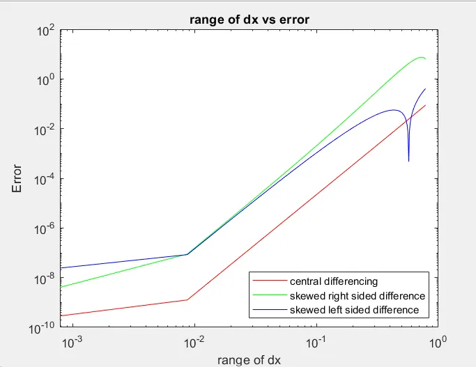
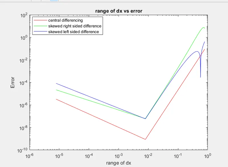
for dx= pi/4 to pi/40000000 with 100 divisions

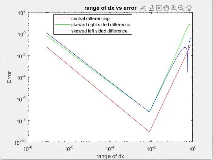
Total error= Truncation error + Round-off error

Comparing the above three plots we can say that as the dx range value increased the error also increased. Thus, it can be concluded that the increase in the accuracy of truncated error will also lead to increase of total error as round-off error increases due to addition of extra terms.

Advantage of a skew scheme over central differencce scheme:

In cases where it is needed to calculate higher-order derivatives at boundary or corner points, especially when we have flow data on just one side of the domain, the skewed scheme to be quite handy. This choice becomes necessary because the central difference scheme relies on data from both sides of the corner, which might not be accessible in such situations. It's worth noting that while the skewed scheme might not provide the same degree of accuracy as the central difference scheme, it does manage to yield results that fall within an acceptable range of precision.

CONCLUSION:

• The fourth-order differencing methods are notably more accurate than the first-order approaches like FDS and BDS. For larger dx values, errors across all schemes are similar. However, as dx decreases, fourth-order approximations approach the exact values rapidly, while FDS and BDS errors remain relatively constant. Thus, higher-order approximations are significantly more precise.
• Comparing fourth-order schemes, the skewed difference scheme yields the lowest errors, which decrease with smaller dx values. In contrast, central difference scheme errors become constant after a certain point, as observed in all figures.
• Among the fourth-order approximations, central differencing outperforms skewed computations because it considers data from both sides (previous and next nodes) for derivative computation, while skewed schemes only use data from one side, which is less accurate for derivative calculation.