Week 5.1 - Mid term project - Solving the steady and unsteady 2D heat conduction problem

1. AIM:

To perform steady-state analysis and transient state analysis by solving the 2D heat conduction equation using point iterative techniques, with the following boundary conditions:

1. Top Boundary = 600 K
2. Bottom Boundary = 900 K
3. Left Boundary = 400 K
4. Right Boundary = 800 K

The implementation will include the following methods for solving implicit equations:

1. Jacobi
2. Gauss-Seidel
3. Successive Over-relaxation

The convergence criteria for absolute error will be set at 1e-4.

2. SOLUTION:

Steady-state heat conduction:It means that the temperature of a material doesn't change over time at any specific point within that material. In other words, the temperature only depends on where you are in the material and doesn't fluctuate with time.

The mathematical formula for steady-state heat conduction without any heat being generated is expressed as follows:

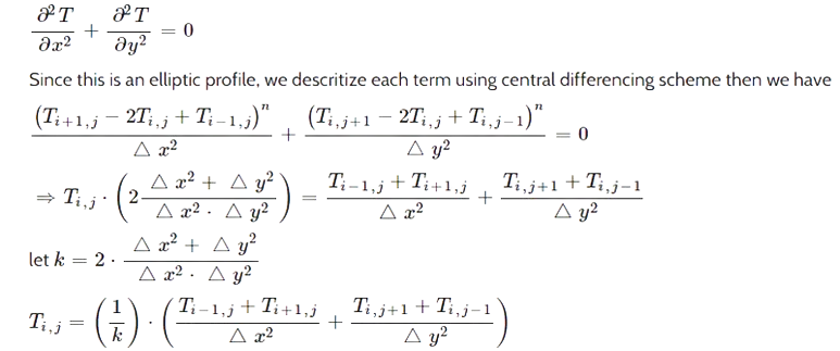
The Jacobi method is a valuable tool in solving complex systems of linear equations, often found in mathematics, engineering, and computer science. Here's a simplified breakdown: To start, make an educated guess for the variables in  equations. Then, update each variable based on the others' current values, using rearranged equations. Repeat this process until the variable values hardly change or meet a specific accuracy level you set. When they stabilize, you've successfully solved the equations. It's like piecing together a puzzle, iteratively refining your solution until it fits just right.

Jacobi method:

Function code for steady-state analysis of 2-D heat conduction equation using jacobii method:

%% steady-state analysis of 2-D heat conduction equation using Gauss-seidel method
function [g,l]=jacobi_method(dx,dy,nx,ny, temp, error, tol,k)
tempold=temp; %updating temperature matrix
%JACOBI ITERATIVE METHOD
    jacobi = 1; %initialize counter 
    while(error>tol) 
        for i = 2:(nx-1) %nested loop over the x-coordinates (i) of the temperature grid
            for j = 2:(ny-1) %nested loop over the y-coordinates (j) of the temperature grid
                %evaluating the updated temperature at grid point (i, j) using the Jacobi method 
            temp(i,j) = (((tempold(i-1,j)+tempold(i+1,j))/(dx^2))+((tempold(i,j+1)+tempold(i,j-1))/(dy^2)))/k;
            end
        end
        error = max(max(abs(temp-tempold))); %checking for convergence
        tempold = temp; 
        jacobi = jacobi+1; %counter increment
    end
    %output values
    g=temp; %Updated temperature
    l=jacobi; % no of iteration
end

where, n is the current time step and n+1 is the next time step.

For Gauss seidel method:

Function code for steady-state analysis of 2-D heat conduction equation using gauss-seidel method:

%% steady-state analysis of 2-D heat conduction equation using Gauss-seidel method
function [r,p]=gauss_method(dx,dy,nx,ny, temp, error, tol,k)
tempold=temp; %updating temperature matrix
%Gauss ITERATIVE METHOD
  gauss = 1; %initialize counter 
    while(error>tol)
        for i = 2:(nx-1) %nested loop over the x-coordinates (i) of the temperature grid
            for j = 2:(ny-1) %nested loop over the y-coordinates (j) of the temperature grid
    %evalauting the updated temperature at grid point (i, j) using the gauss seidel method.
            temp(i,j) = (((temp(i-1,j)+tempold(i+1,j))/(dx^2))+((tempold(i,j+1)+temp(i,j-1))/(dy^2)))/k;
            end
        end
    error = max(max(abs(temp-tempold))); %checking for convergence
    tempold = temp;
    gauss = gauss+1; %counter increment
    end
%Output values
    r=temp; % updated temperature
    p=gauss; %iteration
end

The Gauss-Seidel method is an effective solver for CFD problems but may require numerous iterations for complex cases. Advanced techniques like the Successive Over-Relaxation (SOR) method can be used to expedite convergence in some scenarios.

Successive over-relaxation:

SOR is enhanced gauss-seidel method where nth time step and n+1 time step is all same.

 Here, omega is the relaxation factor.

Function code for steady-state analysis of 2-D heat conduction equation using SOR method:

%% steady-state analysis of 2-D heat conduction equation using SOR method
function [q,z]=SOR_method(dx,dy,nx,ny, temp, error, tol,k)
tempold=temp; %updating temperature matrix
%SOR ITERATIVE METHOD
w=1.4;% Over relaxation factor
  sor = 1; %initialize counter 
    while(error>tol)
        for i = 2:(nx-1) %nested loop over the x-coordinates (i) of the temperature grid
            for j = 2:(ny-1) %nested loop over the y-coordinates (j) of the temperature grid
            %Evaluating the revised temperature at the grid point (i, j) using the gauss-seidel method.
            temp_gs = (((temp(i-1,j)+tempold(i+1,j))/(dx^2))+((tempold(i,j+1)+temp(i,j-1))/(dy^2)))/k;
              % Evaluating the updated temperature at grid point (i, j)
              % using the SOR method using Over relaxation factor
            temp(i,j)=tempold(i,j)*(1-w)+temp_gs*(w);
            end
        end
    error = max(max(abs(temp-tempold))); %checking for convergence
    tempold = temp;
    sor = sor+1; %counter increment
    end
%output values 
    q=temp; %updated temperature
    z=sor; %no. of iteration
end

Transient State modeling, where we explore both Implicit and Explicit schemes.

Implicit Schemes and Explicit Schemes are numerical methods used in computational mathematics to approximate solutions to time-dependent ordinary and partial differential equations. These methods are indispensable in computer simulations of various physical processes. 

Explicit Schemes: In explicit methods, calculation of the future state of a system is solely based on its current state. Essentially, we leap forward in time from the present. Mathematically, if Y(t) represents the current system state and Y(t+Δt) the state at a later time (with Δt being a small time step), we express this as Y(t+Δt) = F(Y(t)).

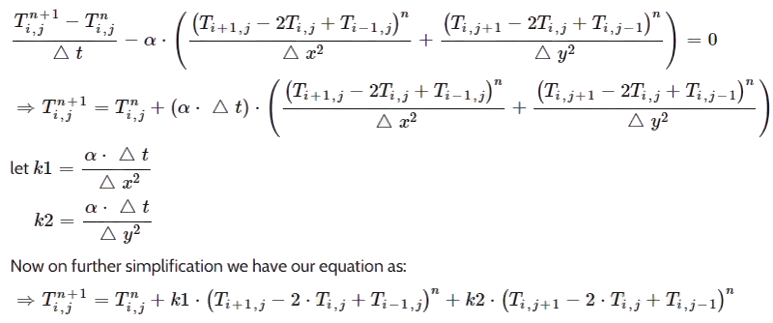
Function code for transient-state analysis of 2-D heat conduction equation (explicit scheme):

%% explixit analysis of 2-D heat conduction equation 
function a = explicit(nt, nx, ny, temp, k1, k2)
    % Initialize the explicit temperature matrix
    tempold = temp;
 exp = 1;
    for p = 1:nt %nested loop for time steps
        for i = 2:(nx-1) %nested loop over the x-coordinates (i) of the temperature grid
            for j = 2:(ny-1)  %nested loop over the y-coordinates (j) of the temperature grid
                term1 = (tempold(i-1,j)-2*tempold(i,j)+tempold(i+1,j));
                term2 = (tempold(i,j-1)-2*tempold(i,j)+tempold(i,j+1));
                temp(i,j) = ((tempold(i,j))+(k1*term1)+(k2*term2));
            end
        end
        
    tempold = temp;
    exp = exp+1; %increment counter
    end

    % Return the final temperature distribution
    a = temp; %updated temperature distribution

end

Implicit Schemes: Conversely, implicit methods involve solving an equation that connects both the current and future states of the system. We don't just leap forward; we solve for the future state considering how it relates to the current one. Mathematically, for an implicit method, we tackle an equation such as G(Y(t), Y(t+Δt)) = 0.

Mathematical derivation:

We begin by applying the first heat conduction equation to a node at a given time, and we rewrite the equation as follows:

Here, we approximate the partial differentials using difference quotients. The temperature term on the right side is approximated using a first-order forward difference quotient, while the second-order partial differential on the left side is approximated with a central difference quotient.

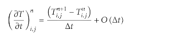
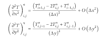
By substituting these values, we derive the difference equation for heat conduction. This equation is essential in simulating heat transfer, with a truncation error of O(Δt + Δx². Δy²).

 

Discretizing the above equation:

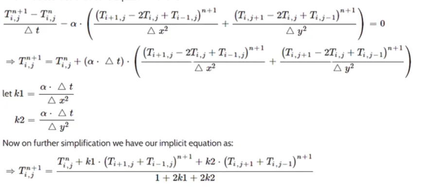
This is the discretized form of our equation. When we apply this discretization to Jacobi, Gauss-Seidel, and SOR methods, we obtain:

Jacobi Method:

Function code for transient-state analysis of 2D heat conduction equation using implicit jacobi method:

%% Transient-state analysis of 2-D heat conduction equation using jacobi method (implicit scheme)
function [b,j] = implicit_jacobi(nt, nx, ny, temp, k1, k2, tol)
    % Initialize the implicit temperature matrix
    tempold=temp;
tprev_dt = tempold;
%d^2(T)/dx^2+d^2(T)/dx^2= 0
% Using Center differencing method at node (i,j)
%JACOBI ITERATIVE METHOD
    jacobi = 1; %initialize counter 
    for k = 1:nt %nested loop for time steps
        error =100;
         while(error>tol)
        for i = 2:(nx-1) %nested loop over the x-coordinates (i) of the temperature grid
            for j = 2:(ny-1) %nested loop over the y-coordinates (j) of the temperature grid
                term1 = (1+(2*k1)+(2*k2))^-1;
                term2 = k1*term1;
                term3 = k2*term1;
                h = (tempold(i-1,j)+tempold(i+1,j));
                v = (tempold(i,j+1)+tempold(i,j-1));
                temp(i,j) = ((tprev_dt(i,j)*term1)+(h*term2)+(v*term3));
            end
        end
        
    error = max(max(abs(temp-tempold))); %checking for convergence
    tempold = temp;
    jacobi = jacobi+1; %counter increment
         end
         tprev_dt = temp ; %updates current temperature distribution for next time step use
    end
    
    % Return the final temperature distribution
    b = temp;
    %iteration value
    j=jacobi;


end

Gauss-Seidel Method

Function code for transient-state analysis of 2D heat conduction equation using implicit Gauss-seidel method:

%% Transient state analysis of 2-D heat conduction equation using Gauss-seidel method (implicit scheme)
function [d,e] = implicit_Gauss_seidel(nt, nx, ny, temp, k1, k2, tol)
    % Initialize the implicit temperature matrix
    tempold=temp; %Initialization
tprev_dt = tempold; 
%d^2(T)/dx^2+d^2(T)/dx^2= 0
% Using Center differencing method at node (i,j)
%GAUSS SEIDEL ITERATIVE METHOD
     gauss = 1; %initialize counter 
    for k = 1:nt  %nested loop for time steps
        error =100; 
         while(error>tol)
        for i = 2:(nx-1) %nested loop over the x-coordinates (i) of the temperature grid
            for j = 2:(ny-1) %nested loop over the y-coordinates (j) of the temperature grid
                term1 = (1+(2*k1)+(2*k2))^-1;
                term2 = k1*term1;
                term3 = k2*term1;
                h = (temp(i-1,j)+tempold(i+1,j));
                v = (tempold(i,j+1)+temp(i,j-1));
                temp(i,j) = ((tprev_dt(i,j)*term1)+(h*term2)+(v*term3));
            end
        end
        
    error = max(max(abs(temp-tempold))); %checking for convergence
    tempold = temp; 
    gauss = gauss+1; %counter increment
         end
         tprev_dt = temp; %updates current temperature distribution for next time step use
    end
    
    % Return the final temperature distribution
    d = temp; %Temperature distribution assigned
    e=gauss; %iteration value assigned


end

Successive Over-Relaxation (SOR) Method

Function code for transient-state analysis of 2D heat conduction equation using implicit SOR method:

%% Transient-state analysis of 2-D heat conduction equation using SOR method(implicit scheme)
function [g,h] = implicit_SOR(nt, nx, ny, temp, k1, k2, tol)
    % Initialize the implicit temperature matrix
    tempold=temp;
tprev_dt = tempold;
%d^2(T)/dx^2+d^2(T)/dx^2= 0
% Using Center differencing method at node (i,j)
%GAUSS SEIDEL ITERATIVE METHOD
    sor = 1; %initialize counter 
    w = 1.2; % Over relaxation factor
    for k = 1:nt %nested loop for time steps
        error =100;
         while(error>tol)
        for i = 2:(nx-1) %nested loop over the x-coordinates (i) of the temperature grid
            for j = 2:(ny-1) %nested loop over the y-coordinates (j) of the temperature grid
                term1 = (1+(2*k1)+(2*k2))^-1;
                term2 = k1*term1;
                term3 = k2*term1;
                h = (temp(i-1,j)+tempold(i+1,j));
                v = (tempold(i,j+1)+temp(i,j-1));
                temp(i,j) = (tempold(i,j)*(1-w))+(w*((tprev_dt(i,j)*term1)+(h*term2)+(v*term3)));
            end
        end
        
    error = max(max(abs(temp-tempold))); %checking for convergence
    tempold = temp;
    sor = sor+1; %counter increment
         end
         tprev_dt = temp; %updates current temperature distribution for next time step use
    end
    
    % Return the final temperature distribution
    g = temp;
    %Iteration value
    h=sor;


end

These techniques play a crucial role in efficiently solving complex transient heat conduction problems, allowing us to explore and understand a wide range of physical phenomena.

 MAIN CODE:

Calling functions and plotting using the main code for all cases:

clear all
close all
clc

% Specify the parameters.
L = 1;
nx = 10;
ny = 10;
dt = 0.01; % Time step
t = 1;
nt = t / dt; % Number of time steps
x = linspace(0, 1, nx);
y = linspace(0, 1, ny);
dx = x(2) - x(1);
dy = y(2) - y(1);

temp = ones(nx, ny);  % Initialization
temp(1, :) = 600; % Top boundary
temp(nx, :) = 900; % Bottom boundary
temp(:, 1) = 400; % Left boundary
temp(:, ny) = 800; % Right boundary

% Establish the corner points by averaging their adjacent values. 
temp(1, 1) = (900 + 400) / 2; % Average temperature of bottom and left boundary
temp(1, 10) = (900 + 800) / 2; % Average temperature of bottom and right boundary
temp(10, 1) = (600 + 400) / 2; % Average temperature of top and left boundary
temp(10, 10) = (600 + 800) / 2; % Average temperature of top and right boundary

alpha = 0.3; % Thermal diffusivity
error = 1;  % error upper limit
tol = 1e-4; % *absolute error criteria
%constant value
k = 2*(dx^2+dy^2)/(dx^2*dy^2);
k1 = (alpha * dt) / (dx^2);
k2 = (alpha * dt) / (dy^2);
%% Invoke the function to perform steady state heat conduction simulation using jacobi method
[f,l]=jacobi_method(dx,dy,nx,ny, temp, error, tol,k);

% Plotting for steady state jacobii
figure(1)
contourf(x,y,f, 'ShowText', 'on');
colorbar;
xlabel('X')
ylabel('Y')
set(gca, 'YDir', 'reverse') %reversing the y axis
text = sprintf('Iteration  = %d', l);
title({'steady state temperature profileby jacobi'; text});

%% Invoke the function to perform steady state heat conduction simulation using gauss-seidel method
[r,p]=gauss_method(dx,dy,nx,ny, temp, error, tol,k);

% Plotting for steady state gauss-seidel
figure(2)
contourf(x,y,r, 'ShowText', 'on');
colorbar;
xlabel('X')
ylabel('Y')
set(gca, 'YDir', 'reverse') %reversing the y axis
text = sprintf('Iteration = %d', p);
title({'steady state temperature profile by gauss-seidel'; text});

%% Invoke the function to perform steady state heat conduction simulation using SOR method
[q,z]=SOR_method(dx,dy,nx,ny, temp, error, tol,k);

% Plotting for  steady state SOR 
figure(3)
contourf(x,y,q, 'ShowText', 'on');
colorbar;
xlabel('X')
ylabel('Y')
set(gca, 'YDir', 'reverse') %reversing the y axis
text = sprintf('Iteration count = %d', z);
title({'steady state temperature profile by SOR'; text});

%% Invoke the function to perform explicit heat conduction simulation
Steady_state_transient_explicit = explicit(nt, nx, ny, temp, k1, k2);

% Plotting for explicit 
figure(4)
contourf(x, y, Steady_state_transient_explicit, 'ShowText', 'on');
colorbar;
xlabel('X')
ylabel('Y')
set(gca, 'YDir', 'reverse') %reversing the y axis
text = sprintf('Iteration count = %d', nt*dt);
title({'Transient state heat conduction profile Explicit'; text});

%% Invoke the function to conduct implicit heat conduction simulations using
% jacobii
[b,j] =implicit_jacobi(nt, nx, ny, temp, k1, k2, tol);

% Plotting for implicit  heat conduction simulation using jacobii
figure(5)
contourf(x,y,b,'ShowText','on');
set(gca, 'YDir','reverse') %reversing the y axis
colorbar;
xlabel('X')
ylabel('Y')
text = sprintf('Iteration count = %d', j);
title({'Transient state heat conduction profile Implicit-Jacobi'; text});

%% Invoke the function to conduct implicit heat conduction simulations using
% Gauss-seidel method
[d,e] = implicit_Gauss_seidel(nt, nx, ny, temp, k1, k2, tol);
%plotting for implicit heat conduction simulation using gauss seidel  
figure(6)
contourf(x,y,d,'ShowText','on');
set(gca, 'YDir','reverse') %reversing the y axis
colorbar;
xlabel('X')
ylabel('Y')
text = sprintf('Iteration count = %d', e);
title({'Transient state heat conduction profile Implicit-Gauss-seidel'; text});

%% Invoke the function to conduct implicit heat conduction simulations using
% Successive over-relaxation method
[g,h] = implicit_SOR(nt, nx, ny, temp, k1, k2, tol);
%plotting for implicit heat conduction simulation using SOR 
figure(7)
contourf(x,y,g,'ShowText','on');
set(gca, 'YDir','reverse') %reversing the y axis
colorbar;
xlabel('X')
ylabel('Y')
text = sprintf('Iteration count = %d', h);
title({'Transient state heat conduction profile Implicit-SOR'; text});

MAIN CODE EXPLANATION: 

• The code starts by defining various parameters, such as the length of the domain (L), the number of grid points in the x and y directions (nx and ny), the time step (dt), and the total simulation time (t). It calculates the number of time steps nt based on t and dt. It also sets up the spatial grid (x and y) and calculates the grid spacing (dx and dy).
• Initialized a 2D temperature matrix temp with ones of size nx by ny.
• Setting boundary conditions on all four sides of the domain by assigning specific temperature values. The top, bottom, left, and right boundaries have fixed temperatures.
• Calculating constants k, k1, and k2 that are used in the numerical methods. These constants are related to thermal diffusivity and grid spacing.

Calling Functions:

• Calling function called jacobi_method to perform a steady-state heat conduction simulation using the Jacobi method. The result is stored in the matrix f.
• It plots the temperature field using contourf and displays it in Figure 1.
• Calling function called gauss_method to perform a steady-state heat conduction simulation using the Gauss-Seidel method. The result is stored in the matrix r.
• It plots the temperature field using contourf and displays it in Figure 2.
• Calling function called SOR_method to perform a steady-state heat conduction simulation using the Successive Over-Relaxation (SOR) method. The result is stored in the matrix q.
• It plots the temperature field using contourf and displays it in Figure 3.
• Calling function explicit to perform an explicit transient heat conduction simulation. The result is stored in the matrix Steady_state_transient_explicit.
• It plots the temperature field using contourf and displays it in Figure 4.
• Calling a function implicit_jacobi  to perform an implicit transient heat conduction simulation using the Jacobi method. The result is stored in the matrix b.
• It plots the temperature field using contourf and displays it in Figure 5.
• Calling a implicit_Gauss_seidel  function to perform an implicit transient heat conduction simulation using the Gauss-Seidel method. The result is stored in the matrix d.
• It plots the temperature field using contourf and displays it in Figure 6.
• Calling a function implicit_SOR to perform an implicit transient heat conduction simulation using the SOR method. The result is stored in the matrix g.
• It plots the temperature field using contourf and displays it in Figure 7.

3. OUTPUTS:

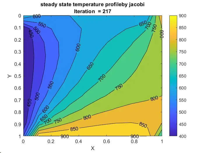
1. Steady state 2D heat conduction using jacobi method:

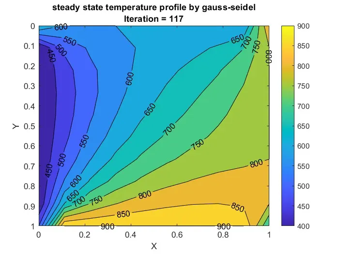
2. Steady state 2D heat conduction using Gauss-seidel method:

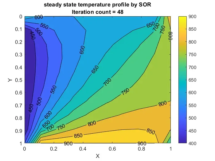
3. Steady state 2D heat conduction using SOR method:

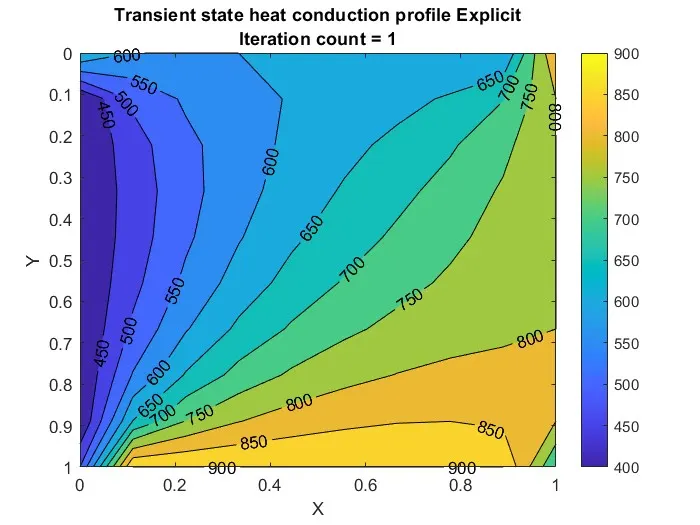
4. Transient state 2D heat conduction using explicit method:

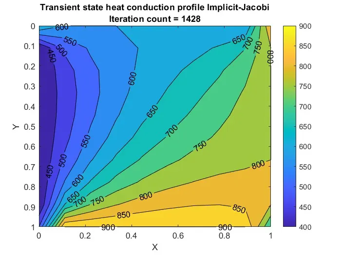
5. Transient state 2D heat conduction using jacobi method:

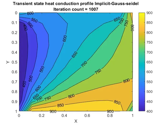
6. Transient state 2D heat conduction using implicit Gauss-seidel method:

7. Transient state 2D heat conduction using Implicit SOR method:

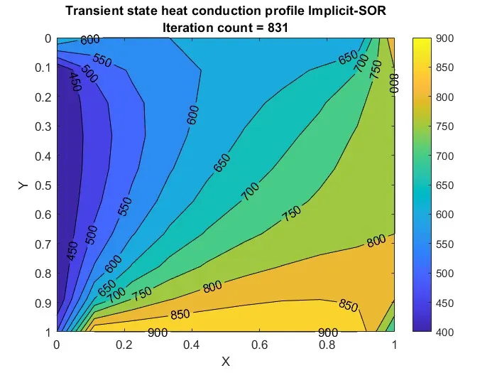
 From the above figure following things can be observed:

• The Successive Over-Relaxation (SOR) method outperformed other techniques in terms of  the number of iterations.
• The findings in steady-state analysis align with those observed previously, highlighting SOR as the superior choice in terms of simulation efficiency.
• Explicit methods exhibited faster convergence when compared to implicit methods.
• In steady-state scenarios, SOR remains the preferred method due to its faster convergence.

Accuracy and Computational Efficiency:

• Explicit methods tend to offer greater accuracy with shorter computational runtimes.
• Comparing the number of iterations across methods and schemes, the order from most to least is: Jacobi > Gauss-Seidel > Successive Over-Relaxation.

Comparison of Steady State and Transient State:

• Steady state simulations consistently require fewer iterations when compared to transient simulations.
• SOR iteration method stands out as the most efficient, requiring the fewest iterations to achieve convergence in both explicit and implicit schemes, surpassing Jacobi and Gauss-Seidel methods.

4. CONCLUSION

 In summary, the Successive Over-Relaxation (SOR) method outperforms other techniques in terms of iteration efficiency, making it the preferred choice for efficient steady-state simulations. While explicit methods show faster convergence, they may sacrifice accuracy. Explicit methods generally offer higher accuracy with shorter runtimes, and the iteration hierarchy is Jacobi > Gauss-Seidel > SOR. In both steady-state and transient simulations, SOR proves the most efficient, requiring the fewest iterations for convergence across both explicit and implicit schemes, surpassing Jacobi and Gauss-Seidel methods. These insights guide method selection in heat conduction simulations, balancing accuracy, computational efficiency, and convergence considerations.