Week 1- Mixing Tee
AIM:
- To perform steady-state simulations to evaluate mixing efficiency when Hot inlet temperature: 36°C, Cold inlet: 19°C.
- To compare k-epsilon and k-omega SST models initially and select the most suitable model for subsequent simulations.
- To run simulations for specified velocity and momentum ratios.
- To compare results for cell count, average outlet temperature, and convergence iterations.
- Generate contour plots for velocity and temperature on cut planes.
- Plot velocity and temperature line plots along and across the pipe.
- To assess solution robustness through a mesh independence study for one case
- To discuss the influence of length and momentum ratio on simulation results.
- Including convergence plots for each simulation to illustrate the convergence process.
Theoretical Background:
Mixing Tees employ a specially designed internal geometry to effectively blend two fluid streams into a unified flow. These tees find optimal use in microbore or analytical gradient High-Performance Liquid Chromatography (HPLC) systems, specifically crafted for high-pressure applications.
In industrial applications, particularly in the petrochemical sector, Mixing Tees play a crucial role in merging two fluid streams with distinct physical and/or chemical characteristics. Challenges arise when significant temperature disparities exist between these streams, potentially causing substantial metal temperature fluctuations at the point of convergence if not properly addressed in the design. Such temperature fluctuations can lead to thermal fatigue in the pressure boundary piping, raising the risk of through-wall cracking, fluid leakage, and, in extreme cases, fire hazards.
Ensuring the stability of the piping system under these conditions is paramount. Options for mitigating risks involve enhancing the mixing process to minimize temperature fluctuations. This can be achieved through redesigning the piping system to favor a favorable momentum ratio for rapid mixing or installing protective devices like injection quills or thermal sleeves in regions with elevated temperature fluctuations beyond a thermal fatigue threshold. This critical region encompasses the T-junction and extends downstream for several to numerous main pipe diameters.
Literature provides empirical correlations to estimate mixing effectiveness and fluid concentration uniformity downstream from the T-junction. These correlations are valuable for determining the length of pipe requiring protection. However, caution is advised when applying them outside the conditions for which they were developed, as they are typically based on experiments using air or water as working fluids, a chemical tracer for mixing uniformity, and small temperature differences between the fluid streams.
For a more accurate assessment of mixing behavior, computational fluid dynamics (CFD) modeling, such as well-resolved large eddy simulation (LES), proves beneficial. This approach yields precise predictions of velocity, concentration, and temperature fields within the mixing tee. By analyzing transient fluid temperature variations, it becomes possible to pinpoint a location in the main pipeline where the maximum temperature difference falls below a specified threshold.
Turbulence Models:
Turbulence modeling involves the development and application of mathematical models to predict the impact of turbulence. Turbulent flows are ubiquitous in real-world scenarios, such as blood flow in the cardiovascular system, airflow over aircraft wings, and the re-entry of space vehicles. Despite extensive research, there is no analytical theory to precisely predict the evolution of turbulent flows. The governing equations for turbulent flows can only be directly solved for simple cases, necessitating the use of turbulence models in Computational Fluid Dynamics (CFD) simulations to predict turbulence evolution. These models are simplified constitutive equations that forecast the statistical progression of turbulent flows.
Several examples of turbulence models are detailed below:
- Spalart–Allmaras Model:
The Spalart–Allmaras model is a one-equation model that solves a modeled transport equation for kinematic eddy turbulent viscosity. It was specifically crafted for aerospace applications involving wall-bounded flows, demonstrating effectiveness in boundary layers subjected to adverse pressure gradients. Its usage is expanding in turbomachinery applications. - k–ε (k–epsilon) Turbulence Model:
The k-epsilon turbulence model is a prevalent choice in CFD to simulate mean flow characteristics in turbulent conditions. This two-equation model describes turbulence through two transport equations, originally developed to enhance the mixing-length model and provide an alternative to algebraically prescribing turbulent length scales. - k–ω (k–omega) Turbulence Model:
The k–omega turbulence model is a common two-equation model used as a closure for the Reynolds-averaged Navier–Stokes equations in CFD. It predicts turbulence using partial differential equations for two variables, k (turbulence kinetic energy) and ω (specific rate of dissipation), offering insights into turbulent flow characteristics. - SST (Menter’s Shear Stress Transport) Model:
The SST turbulence model, a robust two-equation eddy-viscosity model, combines the k-omega and k-epsilon models. It employs k-omega in the inner boundary layer region and switches to k-epsilon in free shear flow, making it versatile for a range of flow conditions. - Reynolds Stress Equation Model:
The Reynolds stress equation model (RSM), also known as the second-moment closure model, stands out as a comprehensive turbulence modeling approach. In contrast to eddy-viscosity-based models, such as k–ε and k–ω, RSM excels in complex engineering flows with high degrees of anisotropy, significant streamline curvature, flow separation, recirculating flow zones, or flows influenced by rotational effects. Eddy-viscosity models fall short in accurately capturing the return to isotropy of turbulence observed in decaying turbulent flows, whereas RSM offers improved accuracy in such scenarios.
K-epsilon (k-ε) vs K-omega (k-ω) turbulence models:
The distinction between the K-epsilon (k-ε) and K-omega (k-ω) turbulence models lies in their predictive capabilities in different regions of the flow field. The K-epsilon model excels in predicting turbulence characteristics away from boundaries (e.g., walls), while the K-omega model performs well in regions near the wall.
In the K-epsilon model, 'k' represents kinetic energy, and 'epsilon' denotes turbulent dissipation, which is the rate at which velocity fluctuations dissipate. However, the model's limitation lies in determining the eddy viscosity from a single turbulence length scale, leading to calculated turbulent diffusion occurring only at that specified scale. This approach may not capture the contribution of all scales of motion to turbulent diffusion, making it less suitable for complex flows involving factors like severe pressure gradients, separation, and strong streamline curvature.
On the other hand, the K-omega model is a two-transport-equation model solving for kinetic energy ('k') and turbulent frequency ('ω'). This model offers improved near-wall treatment by automatically transitioning from a wall function to a low-Reynolds number formulation based on grid spacing. It demonstrates superior performance in wall-bounded and low Reynolds number flows and shows potential for predicting transition phenomena. The K-omega model considers transitional, free shear, and compressible flows.
Problem Setup:
hot inlet Temperature=`36°C + 273.15 = 309.15K`
cold inlet Temperature=`19°C + 273.15 = 292.15K`
Understanding k-epsilon and k-omega SST by considering case-1
Momentum ratio = velocity at cold inlet / velocity at hot inlet
Case-1
Short mixing tee
A)
hot Inlet velocity - 3m/s
Momentum ratio - 2
cold inlet velocity=3*2 =6 m/s
B)
hot Inlet velocity - 3m/s
Momentum ratio - 4
cold inlet velocity=3*4 =12 m/s
Case-2
Long mixing tee
A)
hot Inlet velocity - 3m/s
Momentum ratio - 2
cold inlet velocity=3*2 =6 m/s
B)
hot Inlet velocity - 3m/s
Momentum ratio - 4
cold inlet velocity=3*4 =12 m/s
PROCEDURE:
There are three primary steps involved in conducting any simulation:
- Pre-processor:
This initial phase encompasses geometry cleanup and the generation of a high-quality mesh. Ensuring a refined and accurate representation of the geometry lays the foundation for a successful simulation. - Solving:
The solving phase involves applying boundary conditions, initializing the simulation, and ensuring convergence. Boundary conditions dictate the behavior of the system, and convergence is crucial for obtaining reliable and stable results. - Post-processor:
The post-processing stage includes generating plots, contours, and vectors to analyze the simulation results. Visualization tools provide insights into the simulated phenomena and aid in the interpretation of data.
In the current study focused on assessing the effectiveness of a mixing tee, we will rigorously follow these three steps:
- Geometry Cleanup and Mesh Generation:
This involves preparing the geometry for simulation by addressing any irregularities and generating an optimal mesh for accurate analysis. - Boundary Conditions and Convergence:
Application of appropriate boundary conditions to simulate real-world scenarios, initialization of the simulation, and ensuring convergence for robust and dependable results. - Results Analysis:
Utilizing post-processing tools to generate plots, contours, and vectors that will facilitate a comprehensive analysis of the mixing tee's effectiveness. These visualizations will aid in drawing meaningful conclusions from the simulation data.
Pre-Processing:
Begin by dragging and dropping the mesh setup to load the geometry and initiate the meshing process.
Next, access Space Claim to load the geometry into the setup. Space Claim proves to be a valuable CAD cleanup software, essential for refining CAD geometry in preparation for simulation setups, whether for Finite Element Analysis (FEA) or Computational Fluid Dynamics (CFD).
- Geometry Cleanup using SpaceClaim:
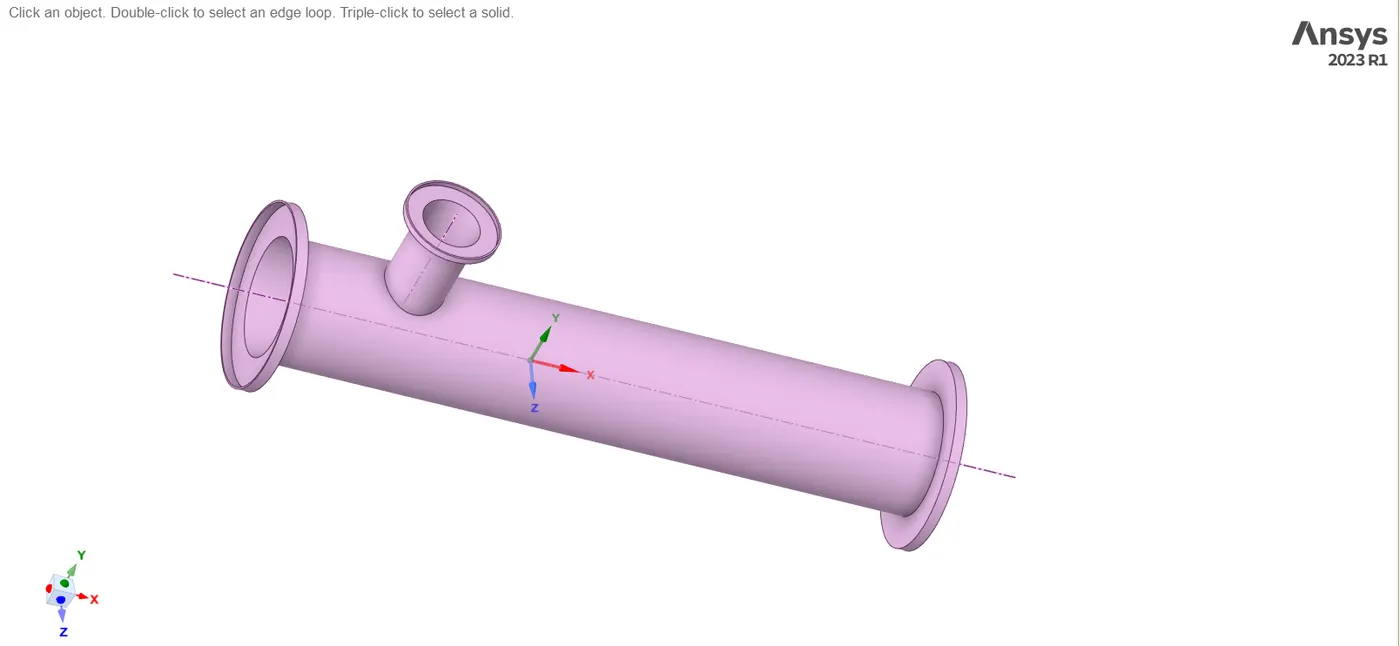
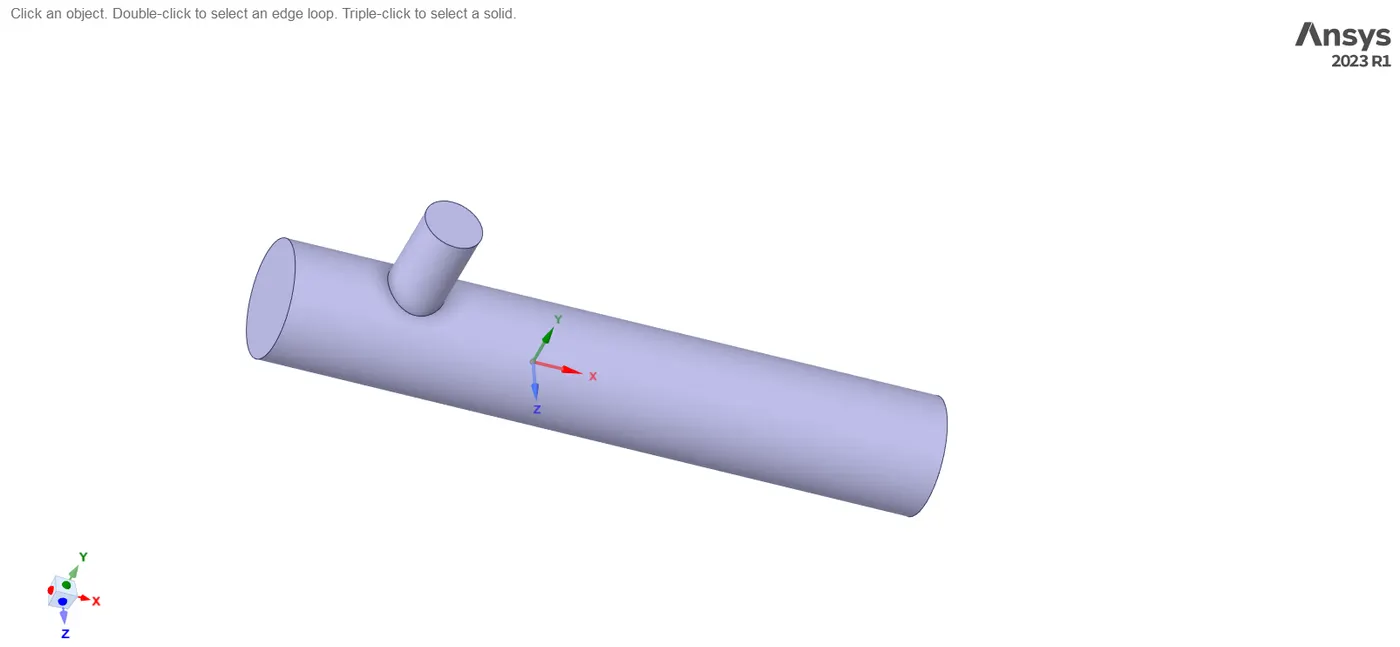
Consequently, load the geometry and proceed to extract the fluid volume, delineating the working fluid volume.
- Mesh Generation:
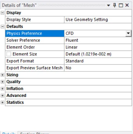
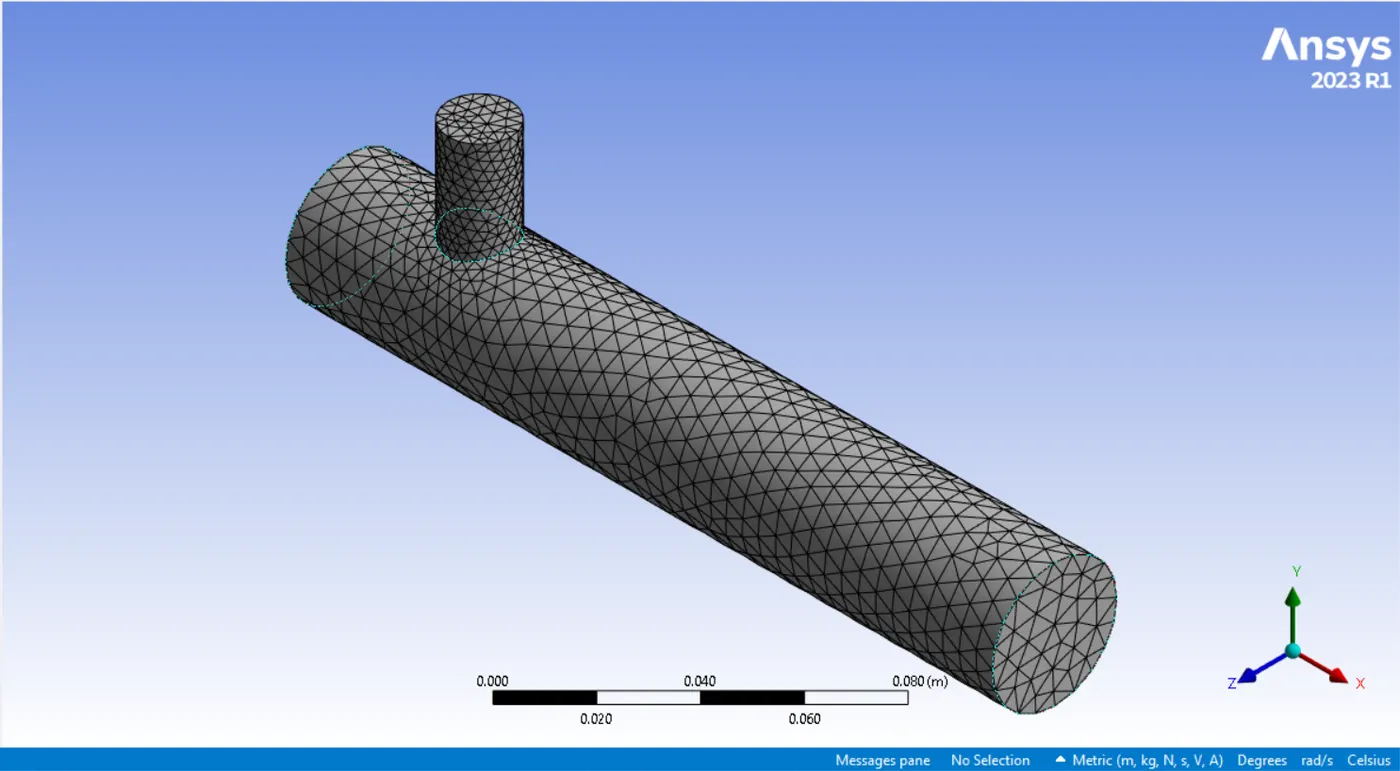
- Element quality:
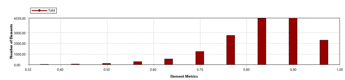
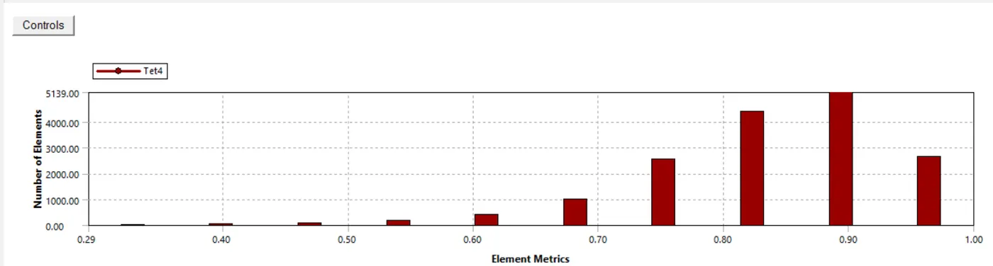
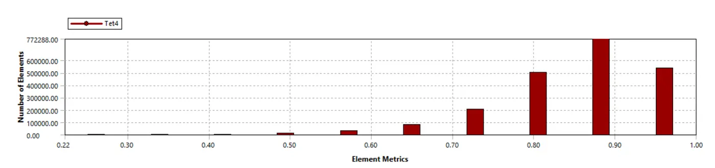
We can check our meshing by cutting the fluid domain into the section as shown below to observe mesh flow. And we can also investigate the quality of mesh by clicking on the option called element quality in the quality section of the mesh panel.
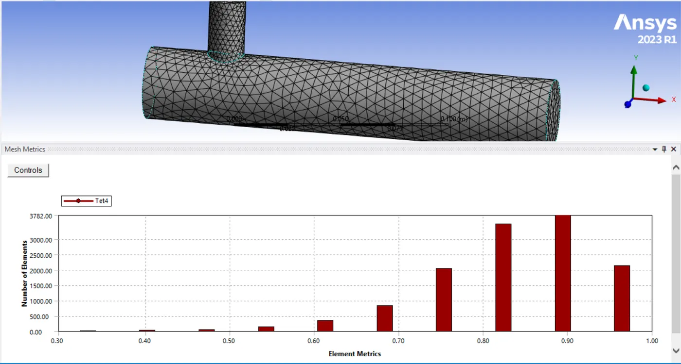
In our graph most of the element are near to 1 so we can say it is good quality.
- Face Naming:
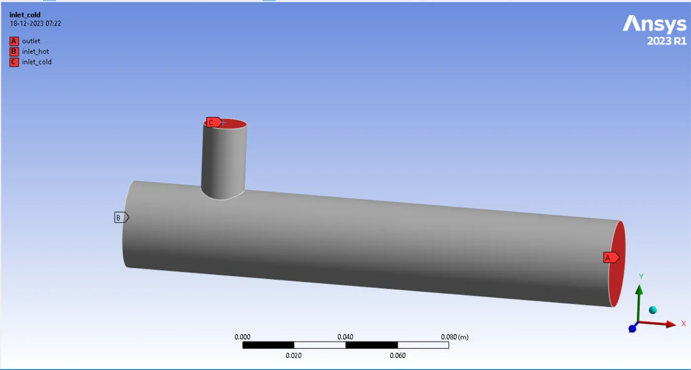
- Solving:
Exit the mesh setup and open the simulation setup. Prioritize the verification of the mesh by ensuring it generates without errors. Only proceed if the mesh validation indicates no errors. In this case, as we are conducting a pressure-based steady-state simulation, select the corresponding options on the task page to align with the simulation objectives.
Solving for case-1 by considering k-epsilon and k-omega SST models.
Considering:
Case-1
Short mixing tee
a)
hot Inlet velocity - 3m/s
Momentum ratio - 2
cold inlet velocity=3*2 =6 m/s
Turbulence model: K-epsilon models.
we will use m2 for momemtum ratio 2 simulation.
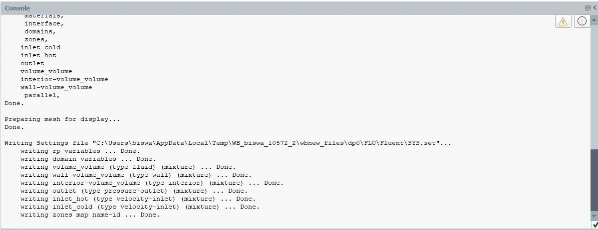
In the Fluent window, the console displays text and accepts TUI (Text User Interface) commands. Initially, it provides information on loading meshing cells and setting boundary conditions in Fluent based on surface names.
Once the entire domain geometry is loaded, it will be visually represented in a user-friendly graphical interface, providing a clear and comprehensive view of how the imported boundary conditions will appear for better user understanding.
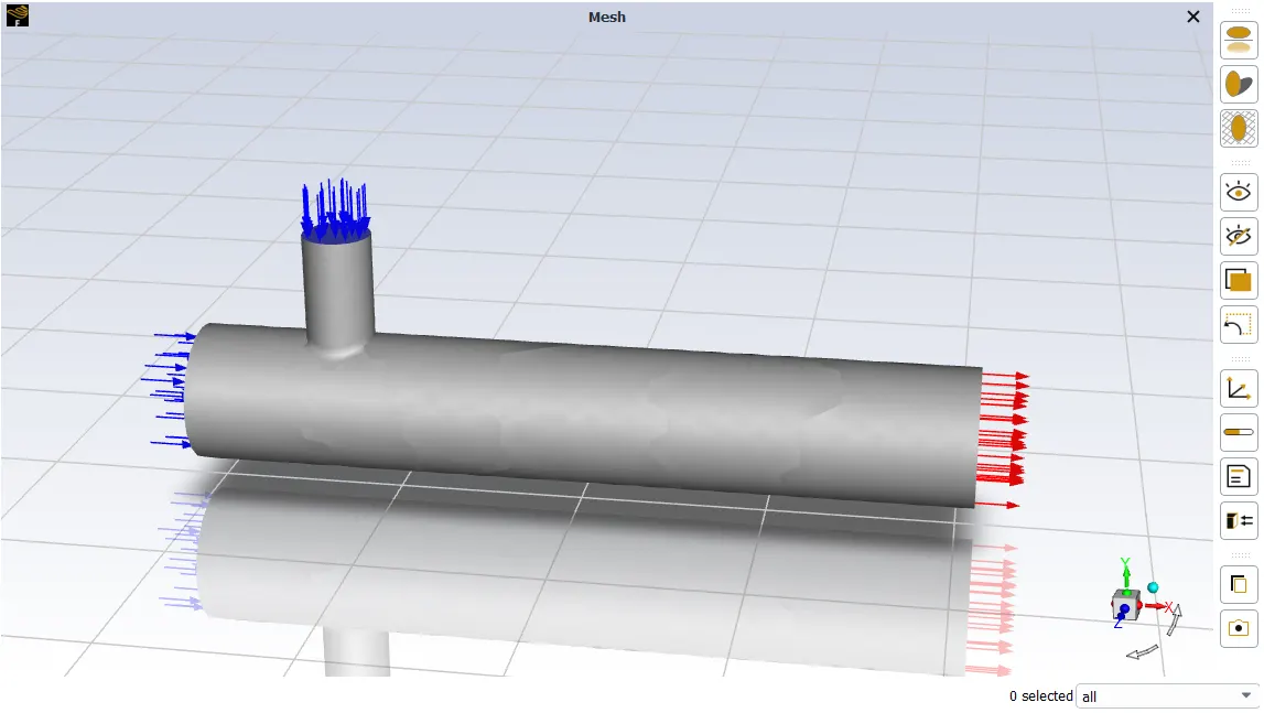
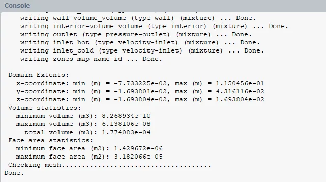
Following this, in the domain panel, the "check" button allows us to assess whether our mesh is suitable for Fluent analysis. Any potential improvements to mesh quality can be made using the "modify" option.
Upon clicking the "check mesh quality" button, the console window provides confirmation, ensuring that each cell is correctly formatted and connected as anticipated. It is crucial to conduct this mesh check immediately after reading it, as any failure in the check indicates a poorly formed or corrupted mesh, necessitating repairs before proceeding with the simulation.
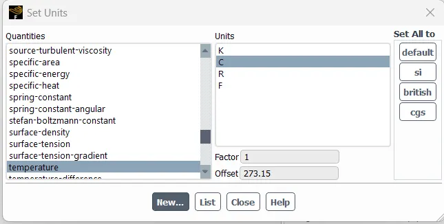
Click ‘units’ to change the units of temperature. FLUENT store values in SI units. Most post-processing can be converted into other units.
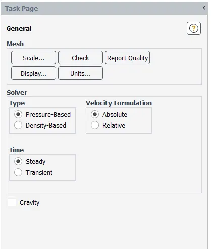
Set the physics of the domain. Keep the general parameter setting as it is. Solver type -> pressure-based; velocity formulation -> Absolute; solver time -> steady.
Next, activate models. First, Turn on the energy Equation. Activating energy equation allows the temperature-dependent problem to be solved.

Viscous Models:
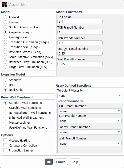
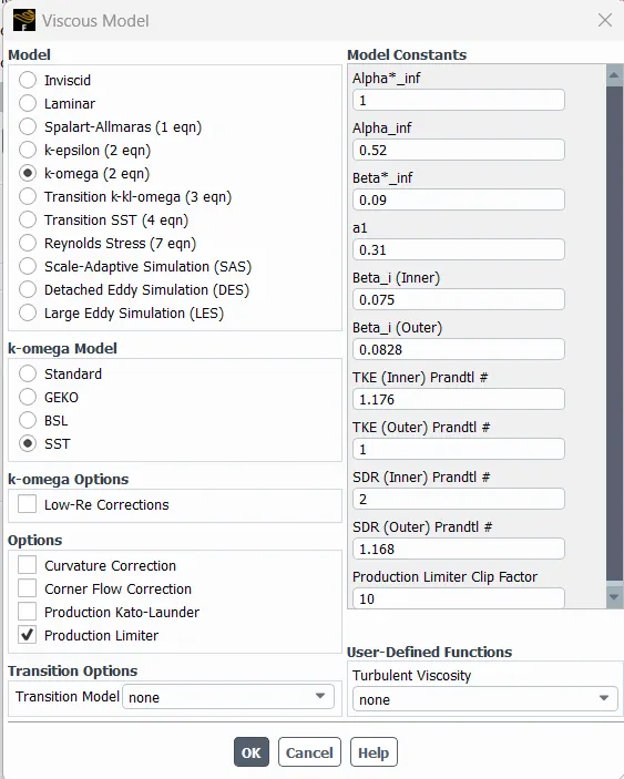
For the viscous model, opt for 'k-epsilon' and 'Realizable' or K-omega SST model for our initial simulation. Turbulence modeling is intricate and varies based on the application.Keep the remaining settings at their default values.
Now follow the same steps as above but use K-omega SST model where required.
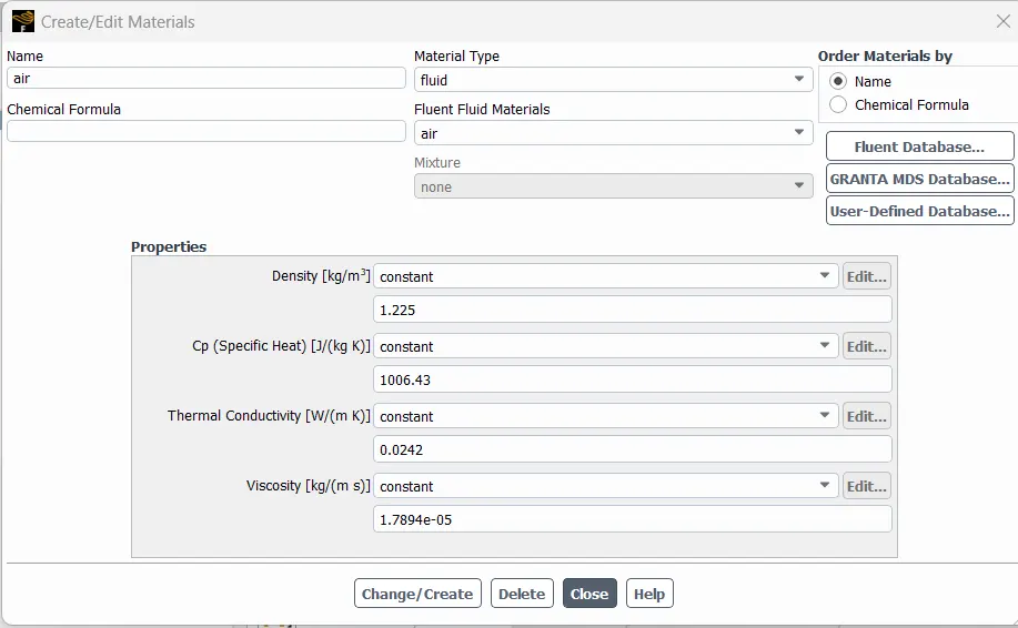
In materials click "FLUENT Database" to add new material. In this case, our working fluid is air so we keep the default material and also in the cell zone define the material, select the working fluid.
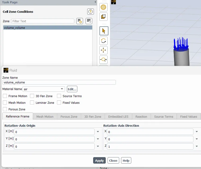
cell zone:
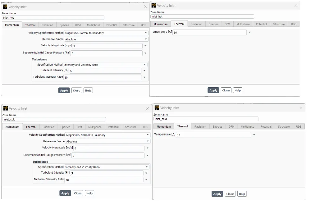
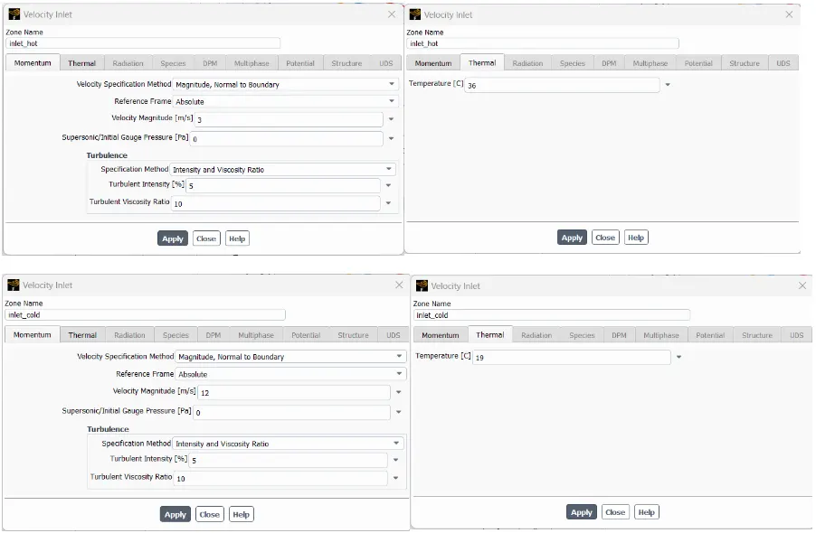
Hot & cold inlet velocity and temperature values:
For momentum ratio 2 use below values:
For momentum ratio 4 use below values:
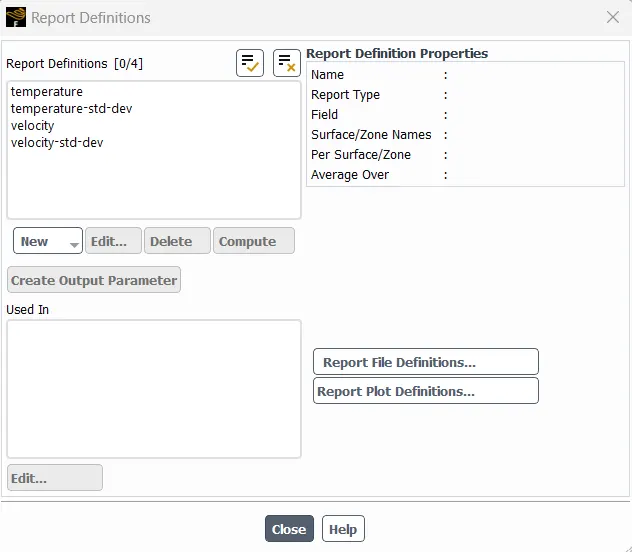
Generate a plot for the average velocity, temperature and their standard deviation at the outlet boundary condition.
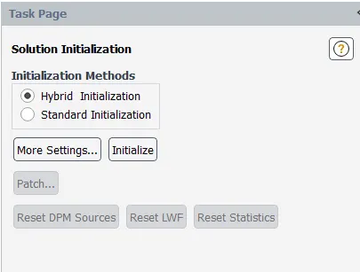
Before executing the program, the final step is to initialize the problem setup.
Initialization establishes the initial solution that the solver will iteratively refine. While generally leading to the same converged solution regardless of initialization, achieving convergence is typically easier when the initial conditions are similar. Basic initialization applies identical values across all cells, and you can enhance this process by patching different values into distinct zones. Some features, such as patching and post-processing, become accessible only after initialization.
The hybrid initialization method is an efficient approach that initializes the solution based solely on the simulation setup, requiring no additional information. This method produces a velocity field conforming to complex domain geometries and a pressure field smoothly connecting high and low-pressure values.
After initialization:
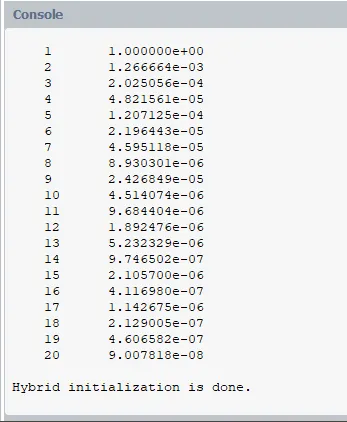
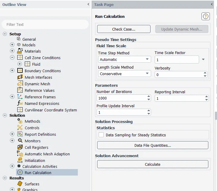
Now, initiate the simulation by entering the desired number of iterations and clicking on the 'calculate' button.
------------------------------------------------------------------------------------------------------------------------------------------------------------------------------------------------------------------------------------------------------------------------------
Case-1 (a)
Results for short mixing K-Epsilon model:
hot Inlet velocity - 3m/s
Momentum ratio - 2
cold inlet velocity=3*2 =6 m/s
Results:
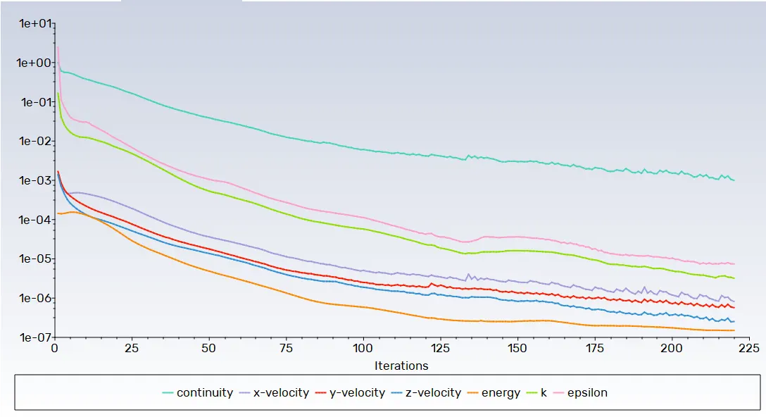
Residual plot:
Standard deviation velocity plot: -
Standard deviation temperature plot: -
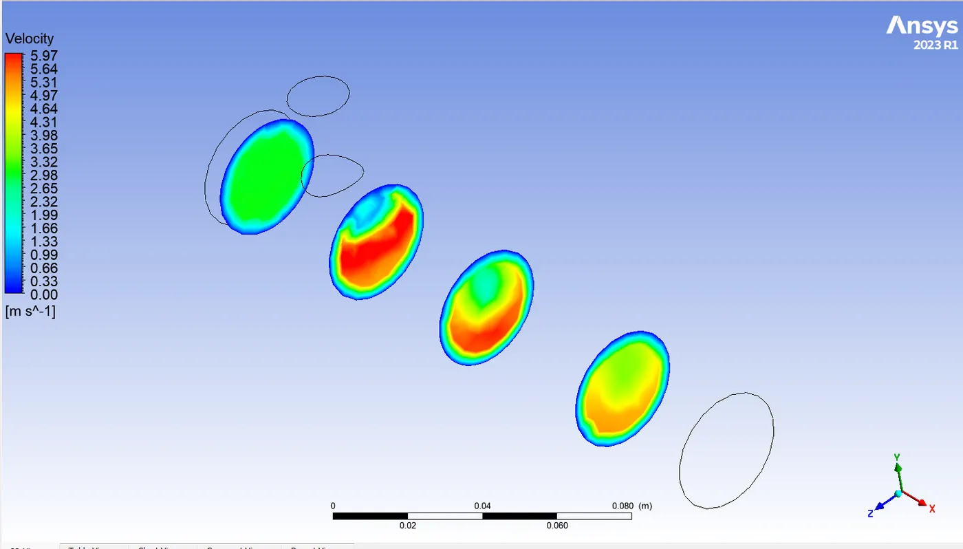
Velocity Contour plot:
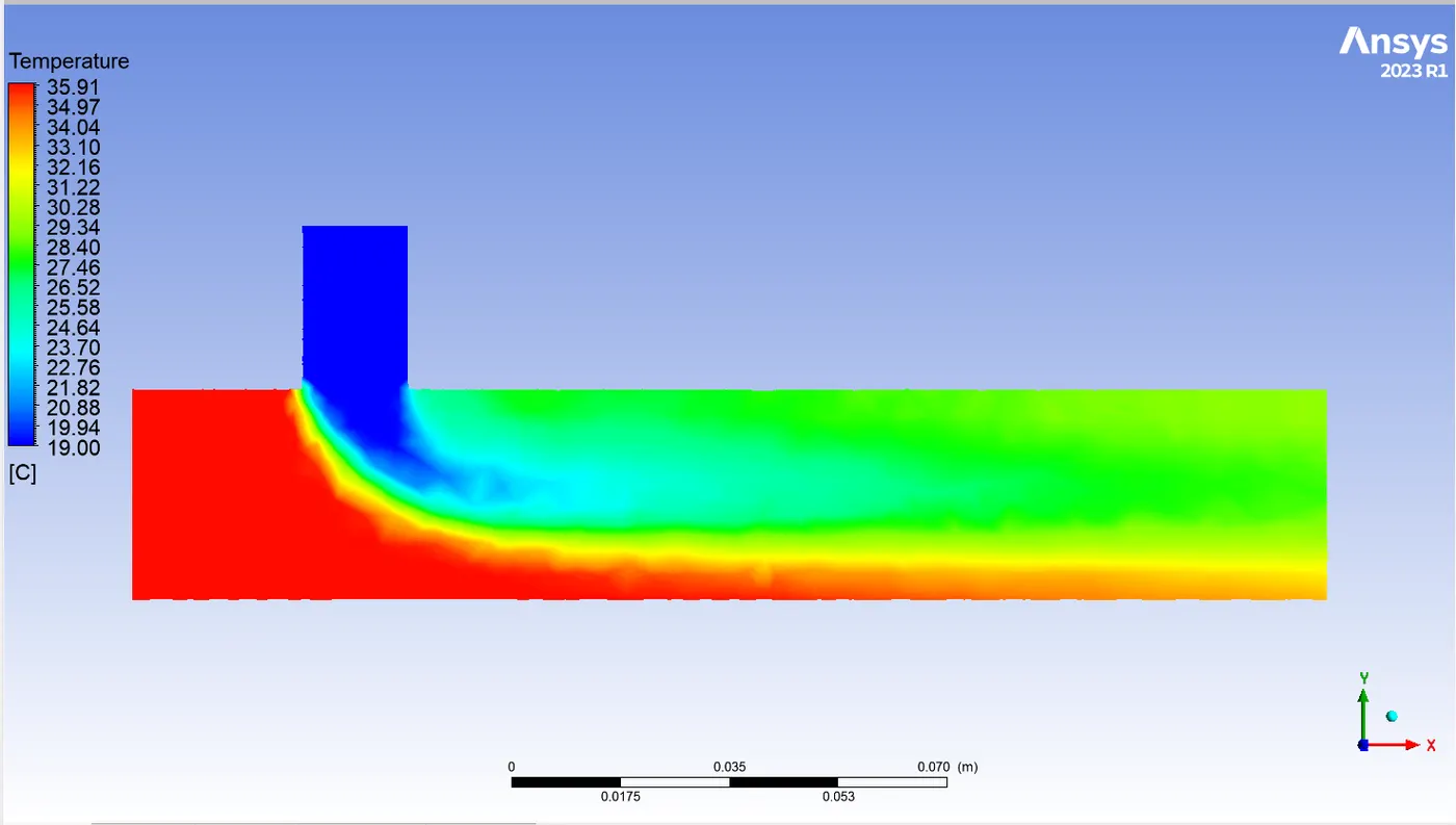
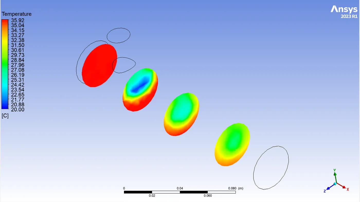
Temperature Contour plot:
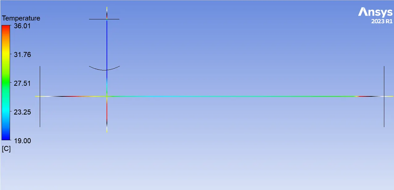
Line Plot:
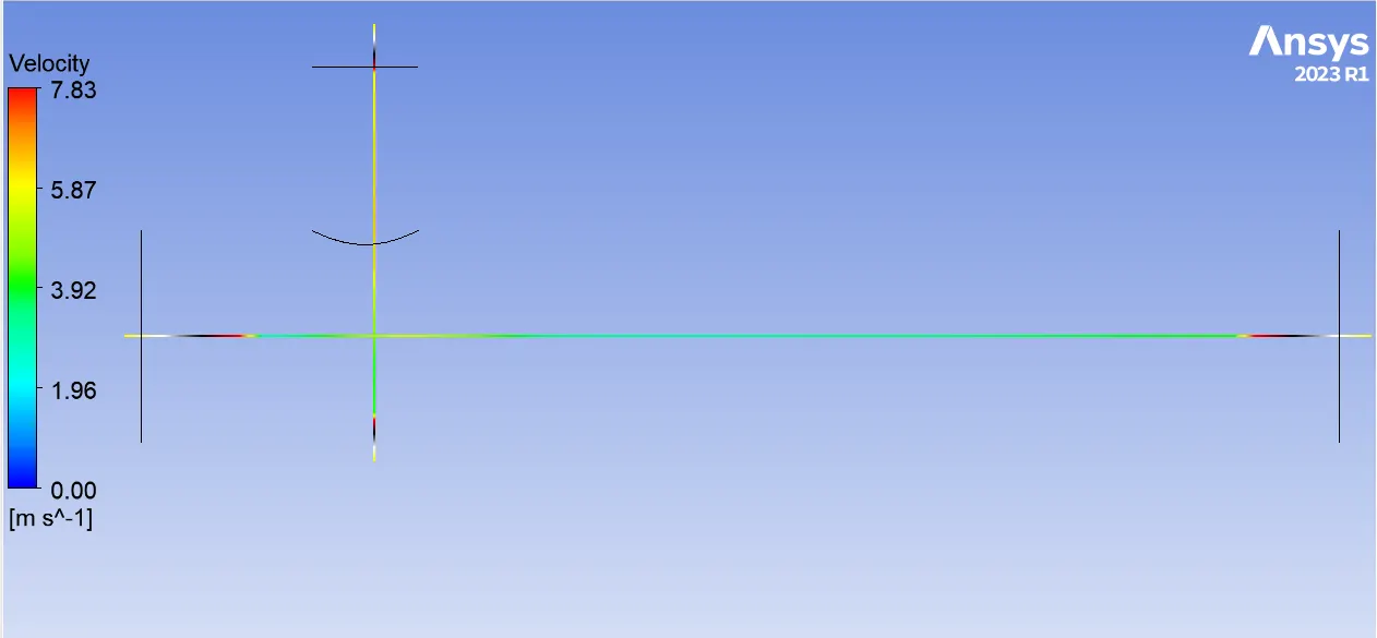
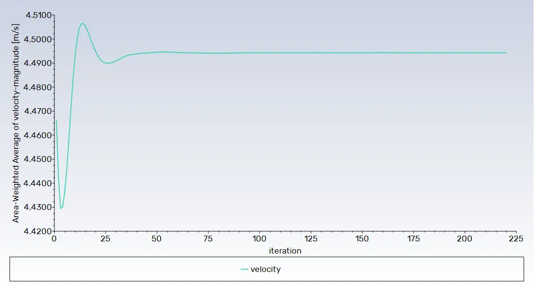
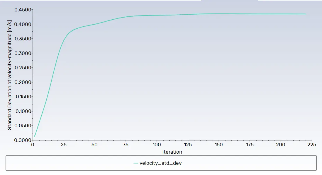
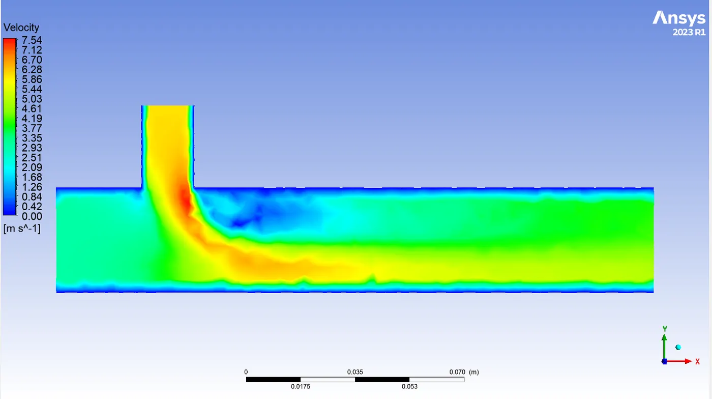
Area Weighted Average velocity at outlet= 4.494292 m/s
Standard Deviation of velocity at outlet=0.19893743 m/s
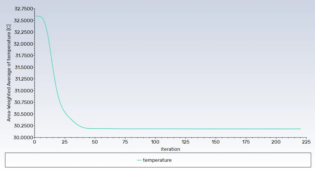
Area Weighted Average Temperature at outlet=30.183071 C
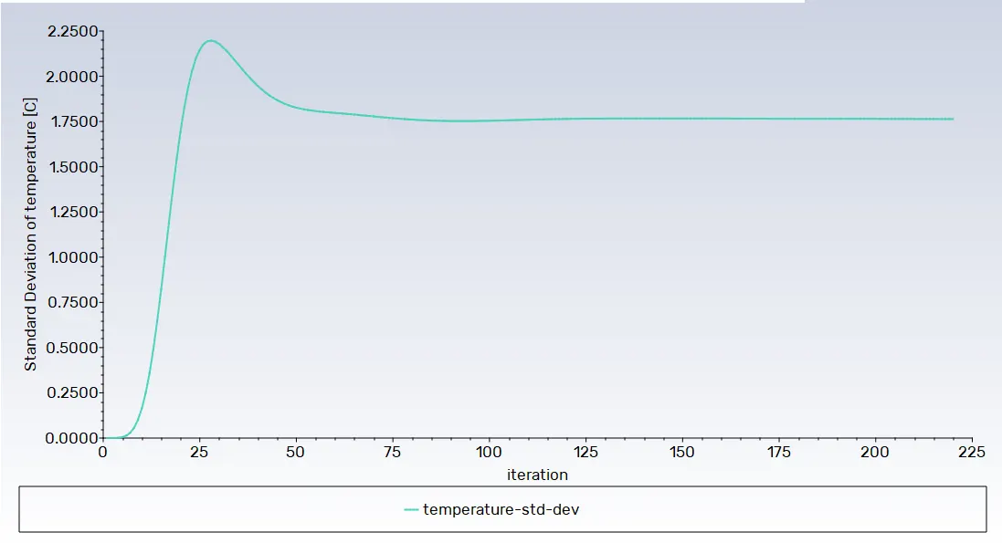
Standard Deviation of temperature at outlet=1.7635359 C
------------------------------------------------------------------------------------------------------------------------------------------------------------------------------------------------------------------------------------------------------------------------------
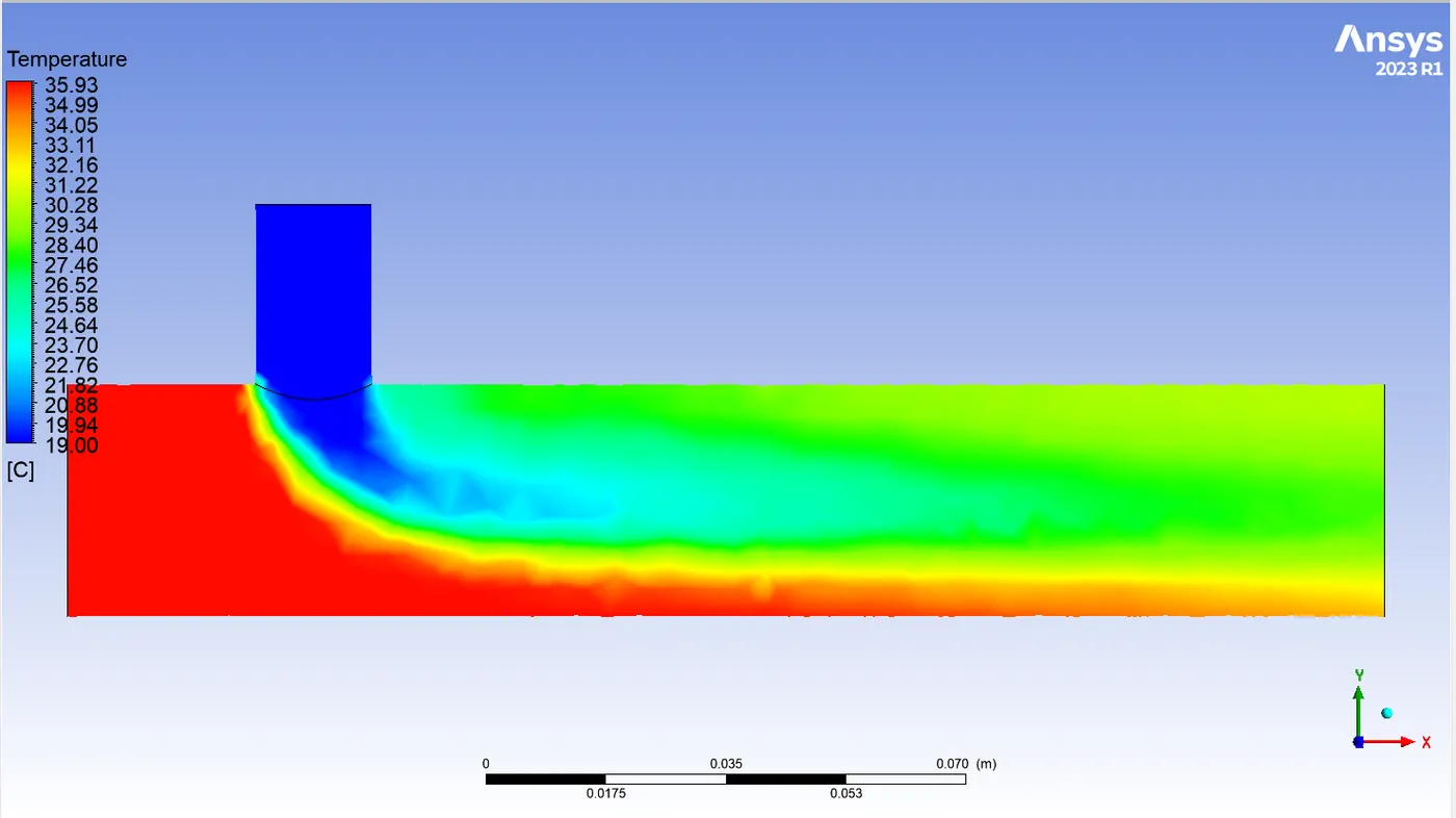
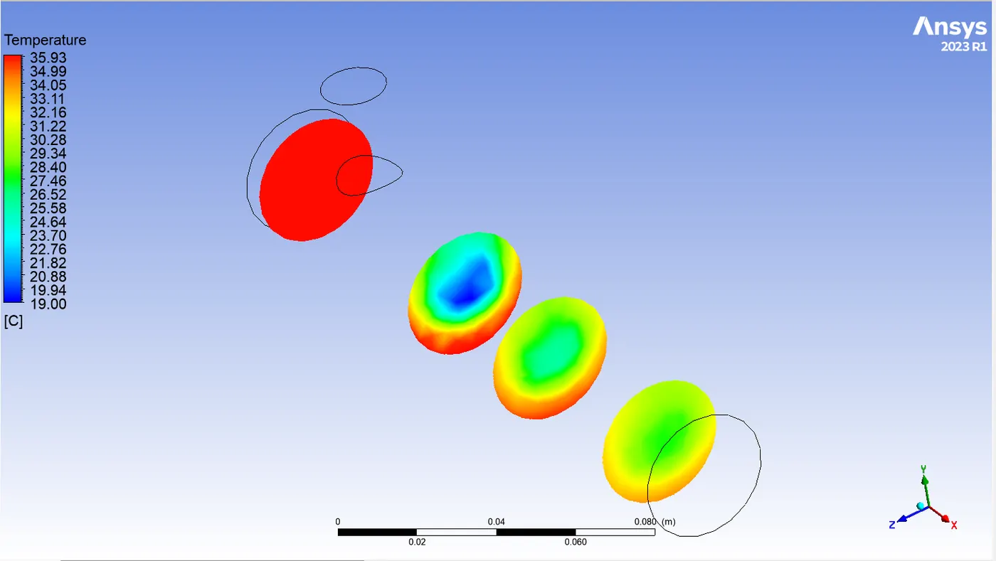
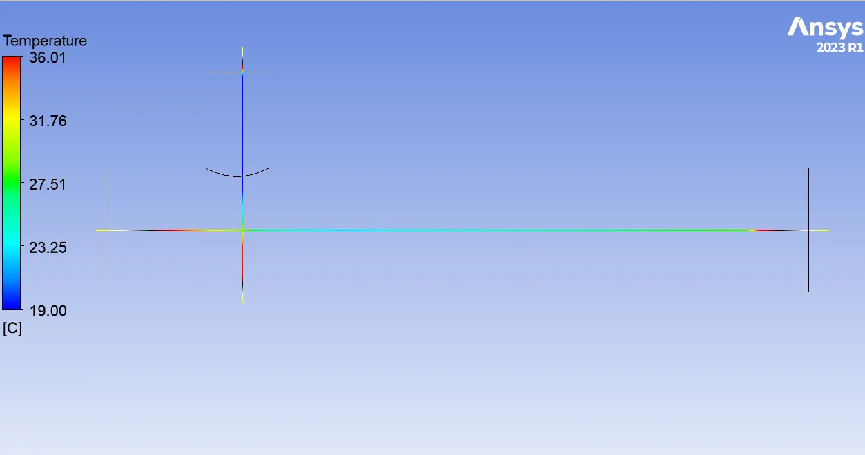
Case 1-a (Turbulence model: K-omega SST model)
hot Inlet velocity - 3m/s
Momentum ratio - 2
cold inlet velocity=3*2 =6 m/s
Results for Short mixing tee:
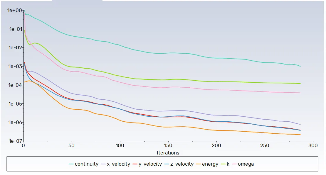
Residual:
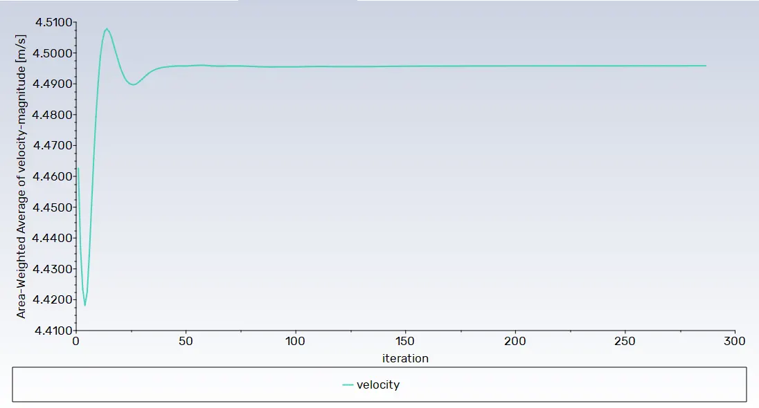
Area weighted average velocity plot:-
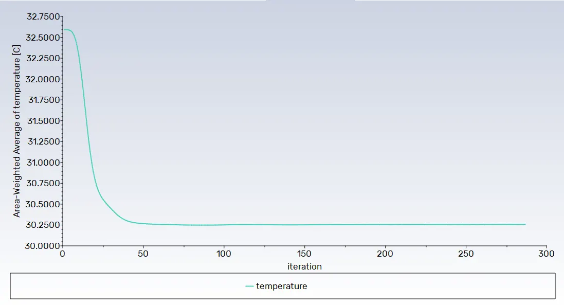
Area weighted average temperature plot:-
Standard deviation temperature plot: -
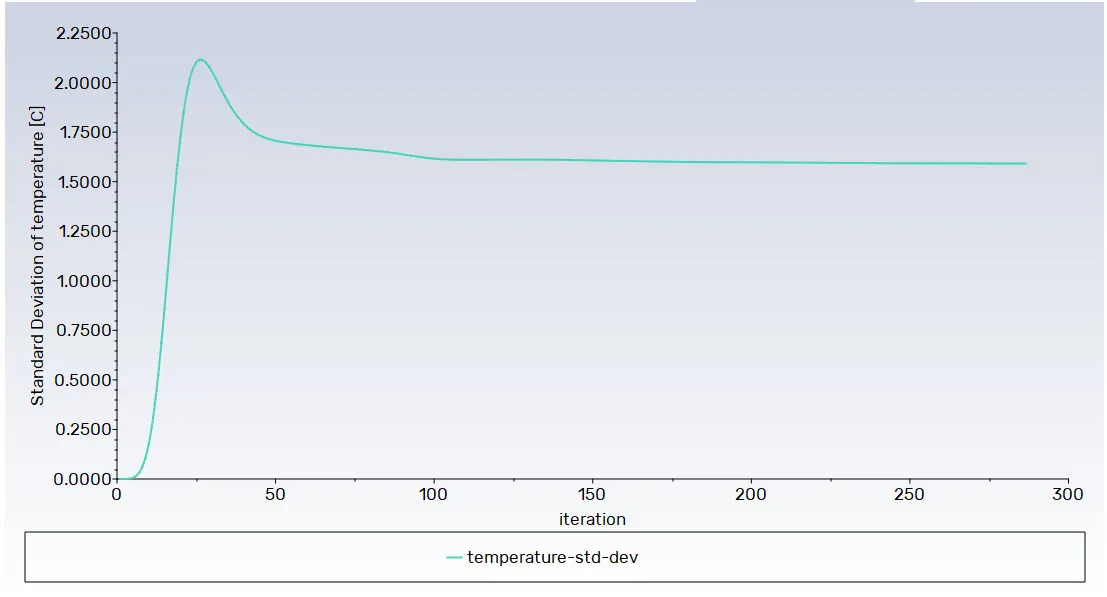
Standard deviation velocity plot: -
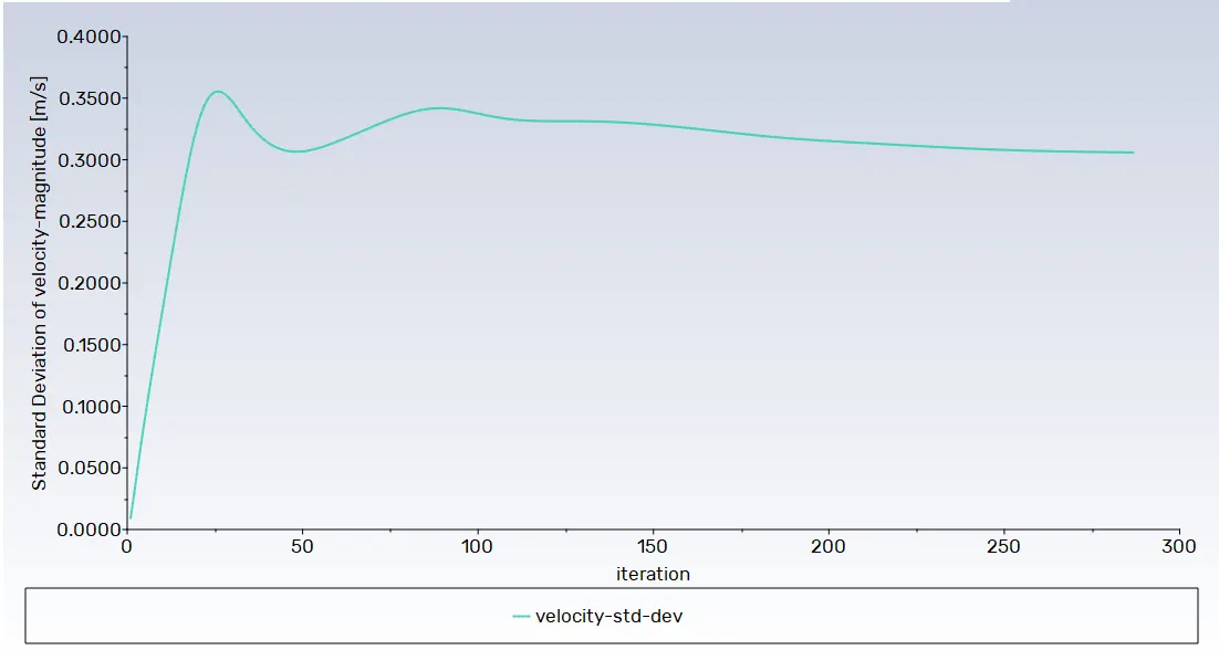
Velocity Contour:
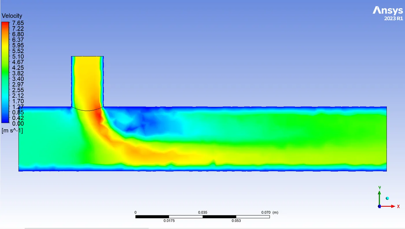
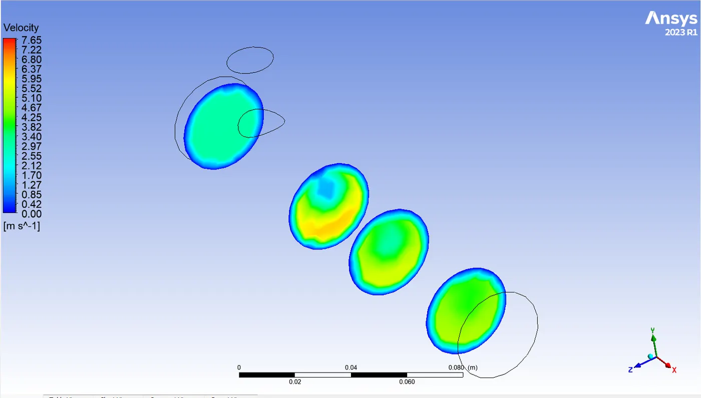
Temperature Contour:
Line Graph:
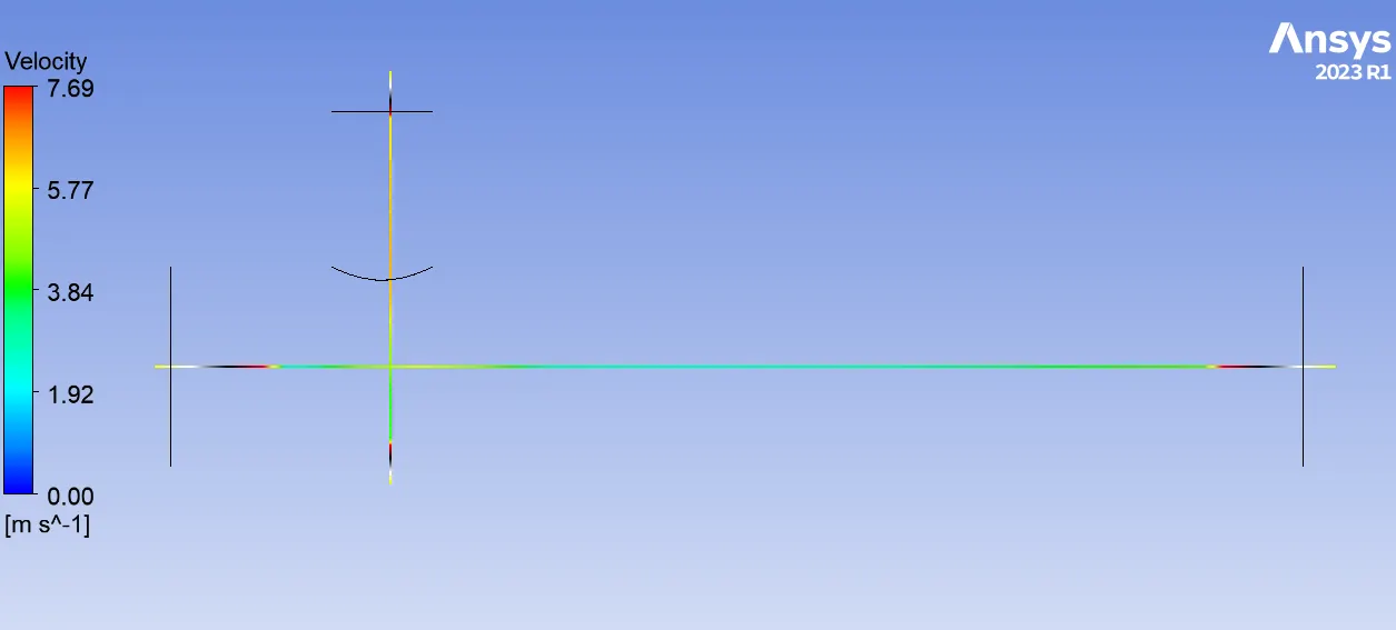
Area Weighted Average velocity at outlet= 4.4958389 m/s
Standard Deviation of velocity at outlet=0.30585978 m/s
Area Weighted Average Temperature at outlet=30.257238 C
Standard Deviation of temperature at outlet=1.5913023 C
------------------------------------------------------------------------------------------------------------------------------------------------------------------------------------------------------------------------------------------------------------------------------
CASE-1-b (Turbulence model: K-Epsilon Realizable)
Hot Inlet velocity - 3m/s
Momentum ratio - 4
cold inlet velocity=3*4 =12 m/s
Lets denote simulation done for momentum ratio=4 as m4
Result for K-Epsilon Realizable:
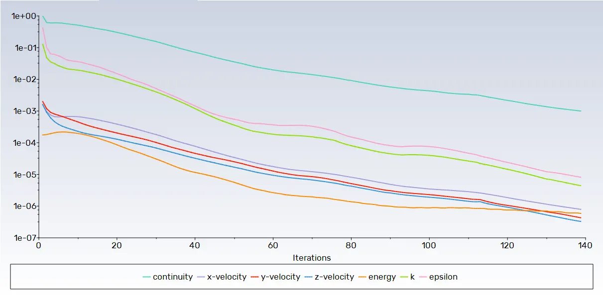
Residual plot:-
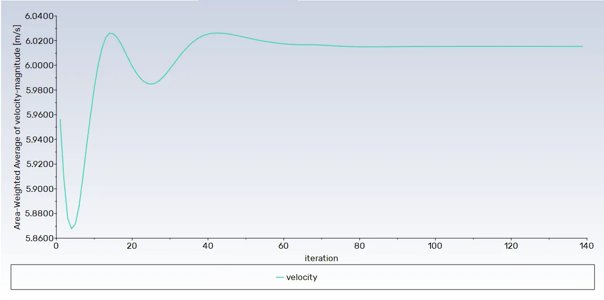
Area weighted average velocity plot:-
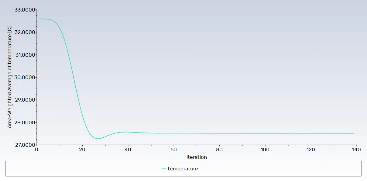
Area weighted average temprature plot:-
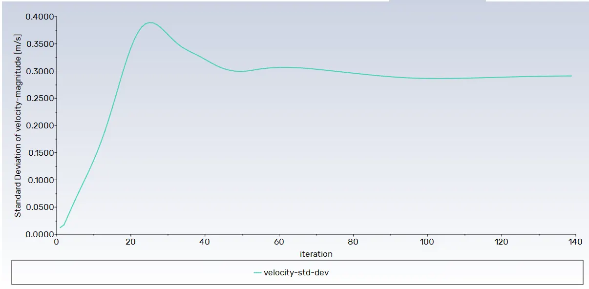
Standard deviation velocity plot: -
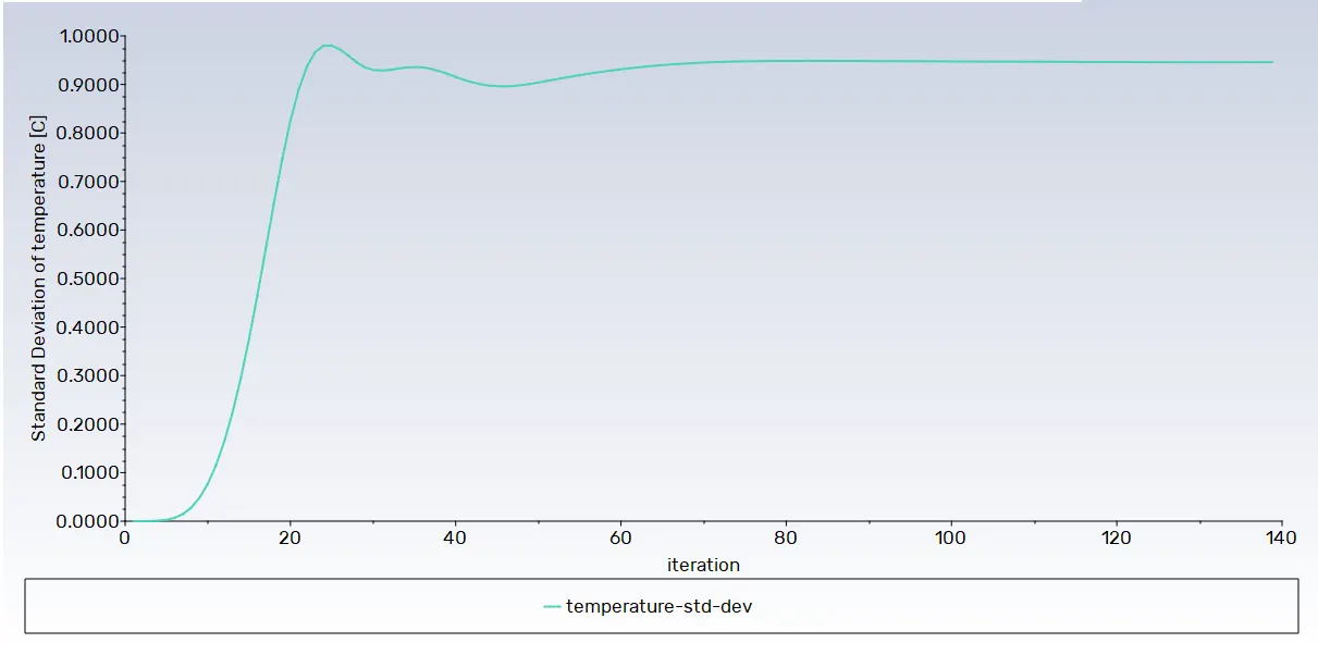
Standard deviation temperature plot: -
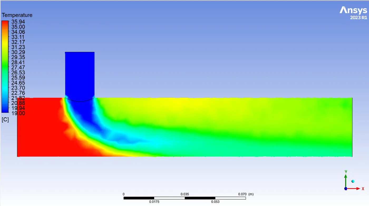
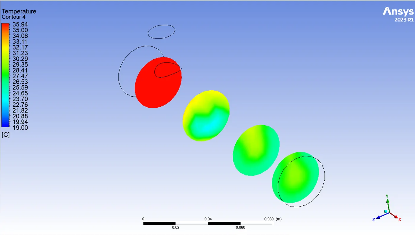
Temperature contour plot: -
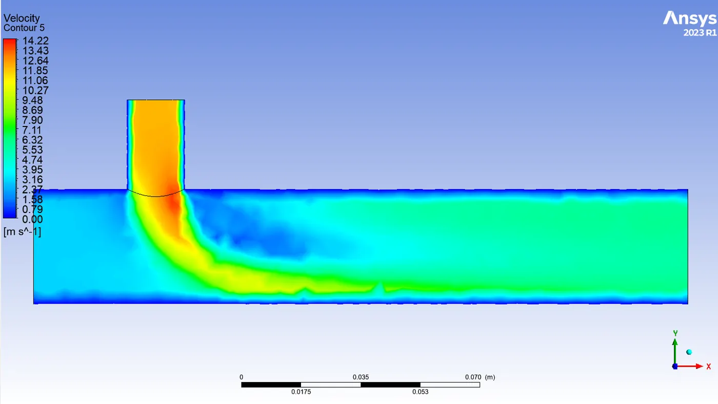
Velocity contour plot:-
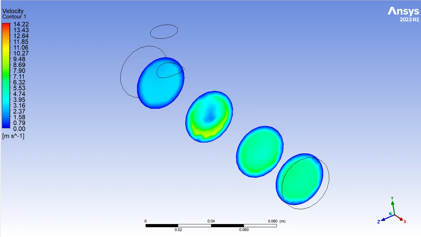
Line Graph:
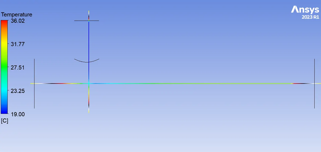
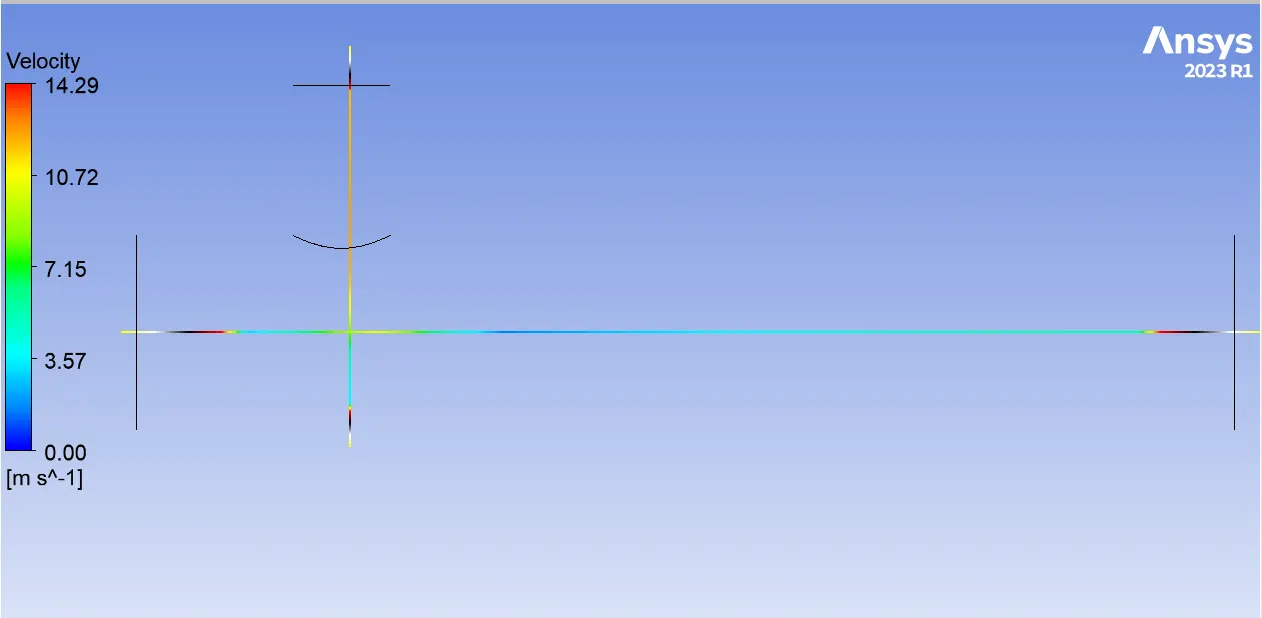
Area Weighted Average velocity at outlet= 6.0152902 m/s
Standard Deviation of velocity at outlet=0.29091446 m/s
Area Weighted Average Temperature at outlet=27.518178 C
Standard Deviation of temperature at outlet=0.94592781 C
------------------------------------------------------------------------------------------------------------------------------------------------------------------------------------------------------------------------------------------------------------------------------
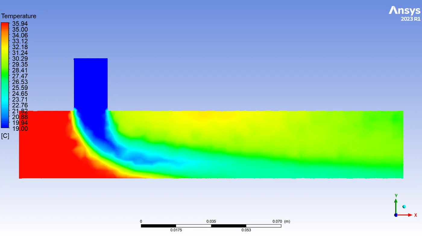
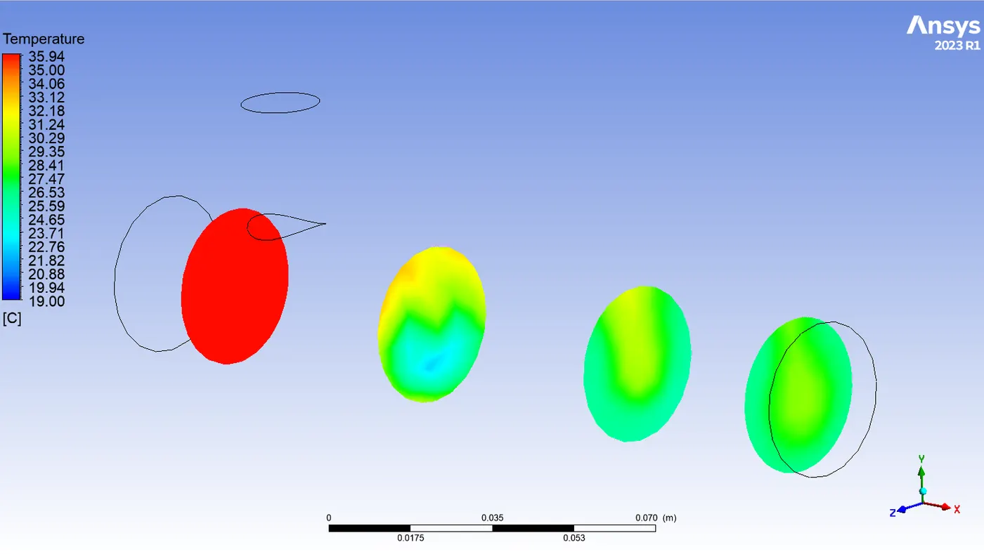
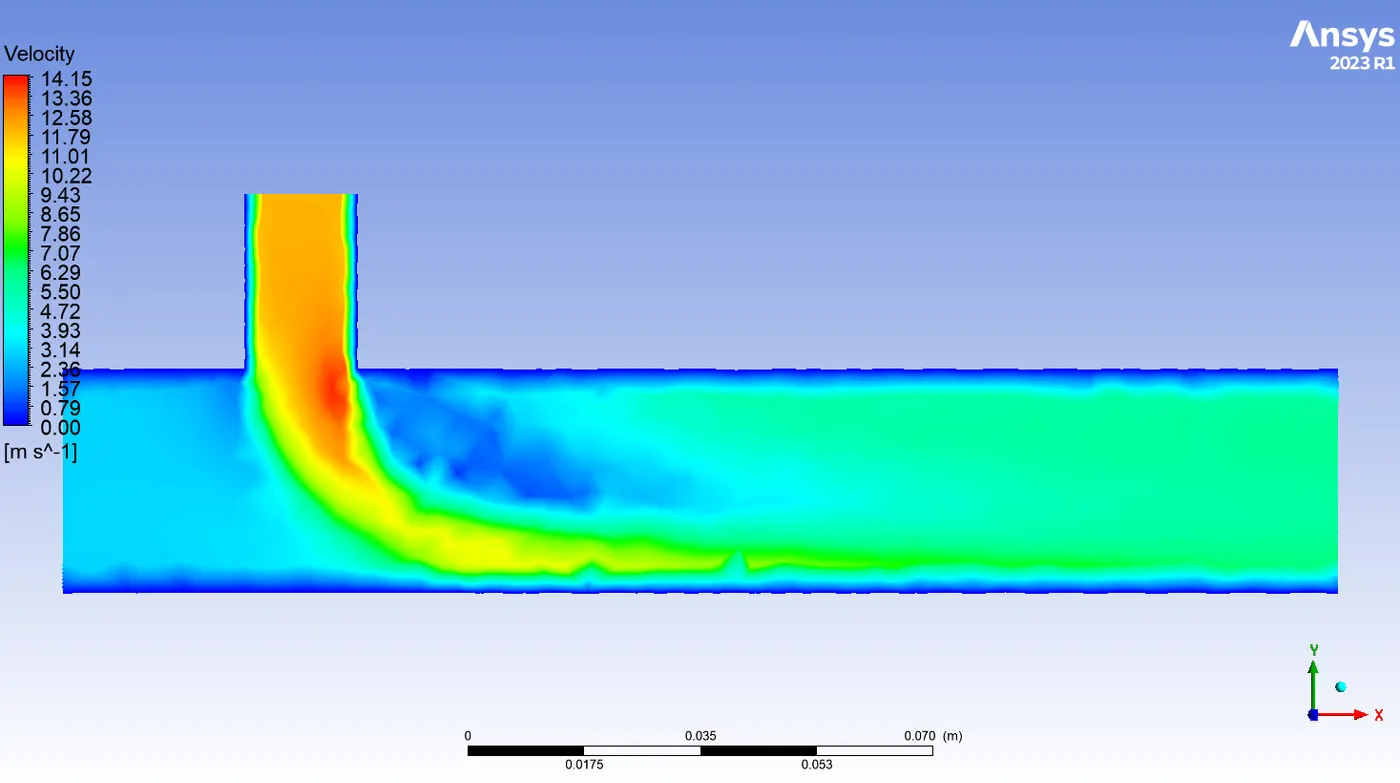
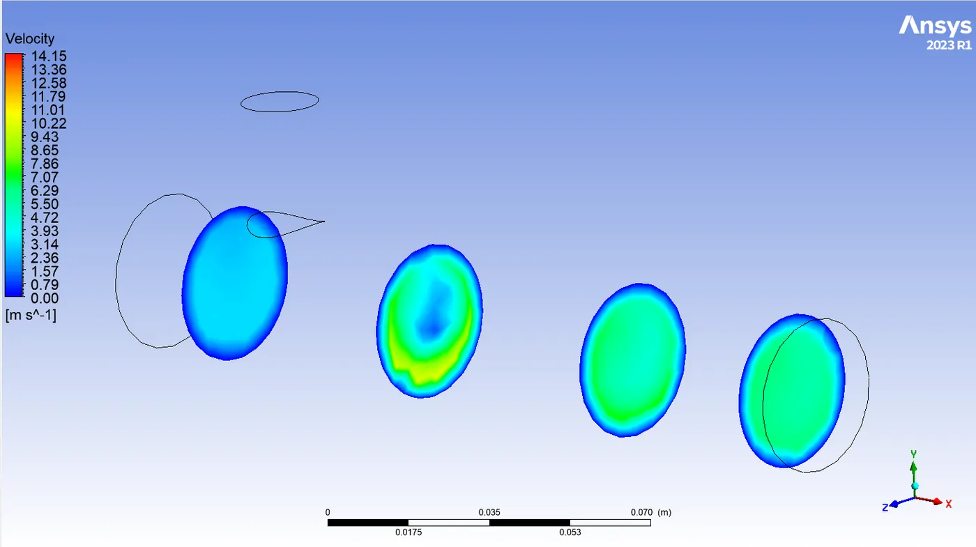
CASE-1-b (Turbulence model: K- omega:)
Hot Inlet velocity - 3m/s
Momentum ratio - 4
cold inlet velocity=3*4 =12 m/s
Lets denote simulation done for momentum ratio=4 as m4
Results:
Residual plot:-
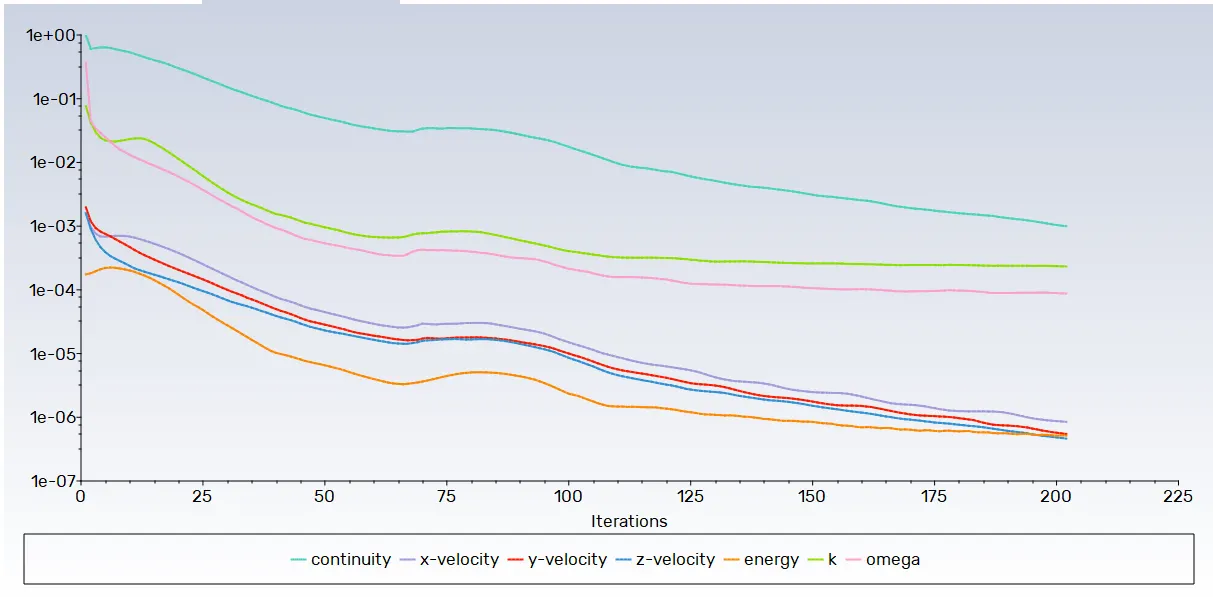
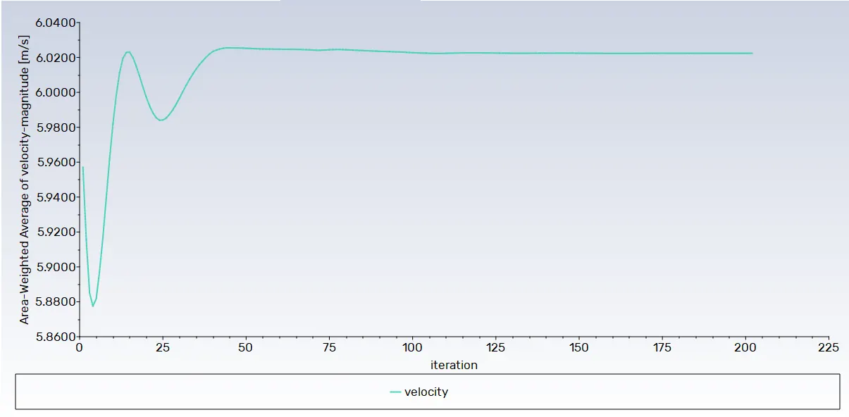
Area weighted average velocity plot:-
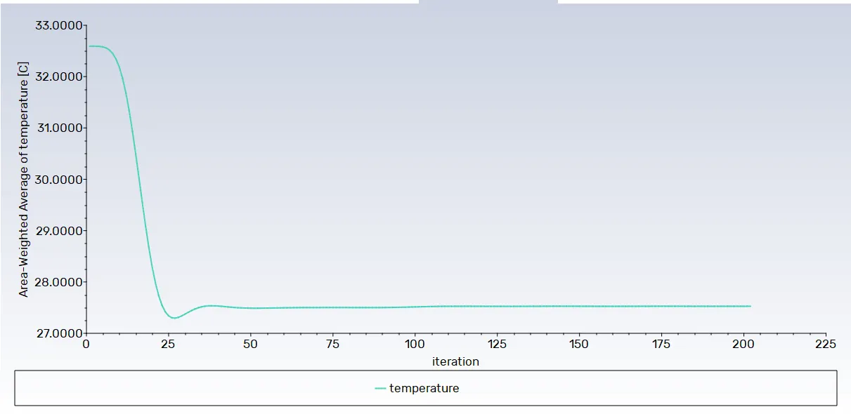
Area weighted average temprature plot:-
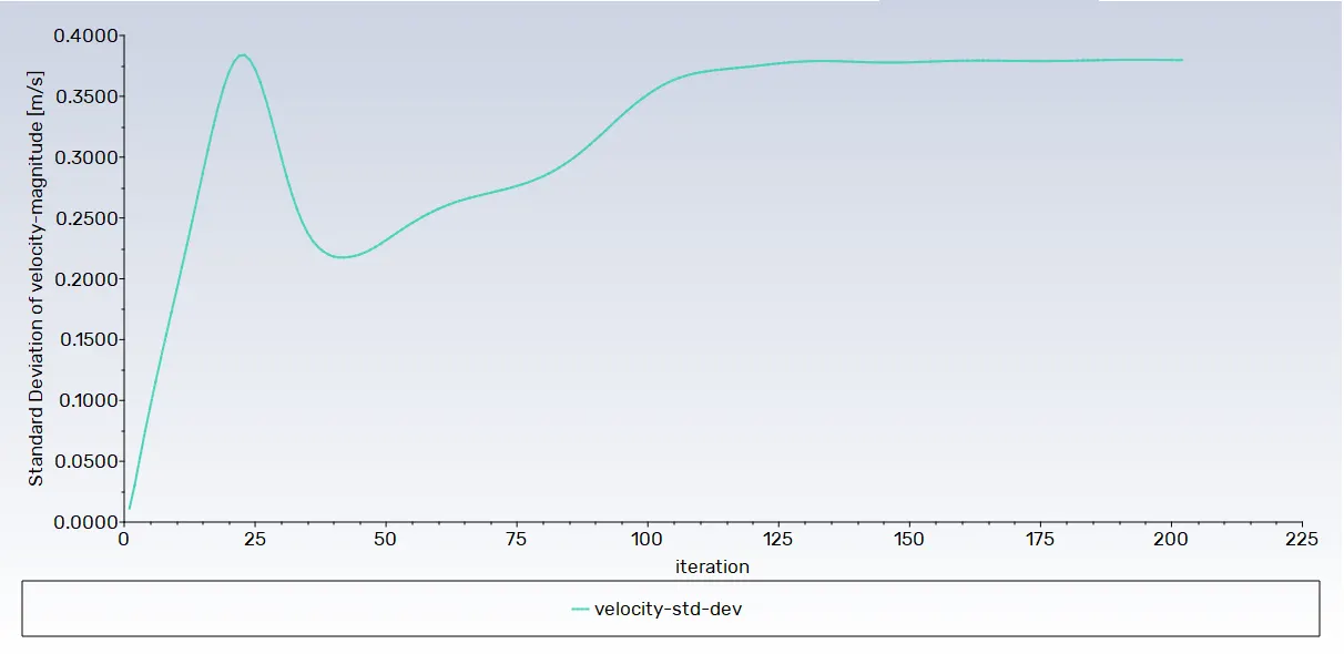
Standard deviation velocity plot: -
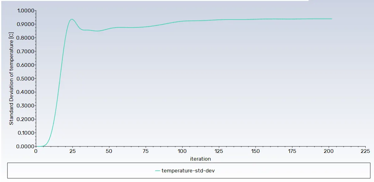
Standard deviation temperature plot: -
Temperature contour plot: -
Velocity contour plot:-
Line Graph:
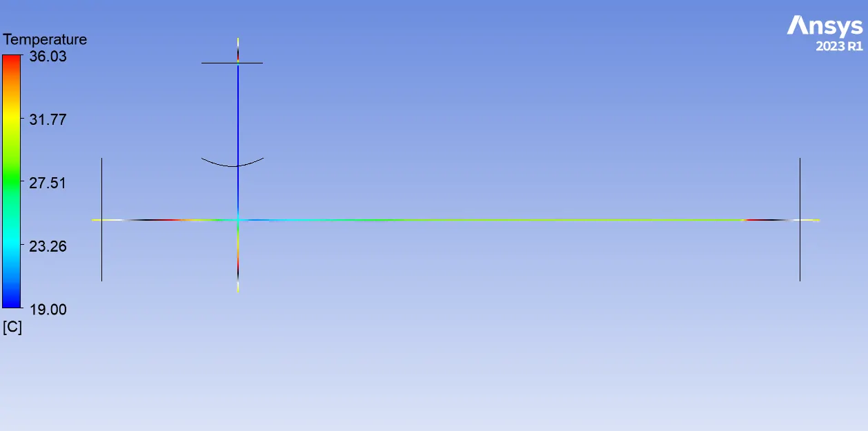
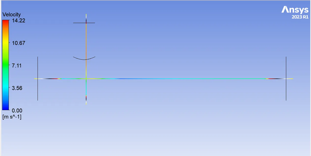
Area Weighted Average velocity at outlet= 6.0223868 m/s
Standard Deviation of velocity at outlet=0.379714 m/s
Area Weighted Average Temperature at outlet=27.527202 C
Standard Deviation of temperature at outlet=0.93887091 C
Based on the above results of case-1 (a&b) study:
The K-epsilon model tends to converge in fewer iterations compared to the K-omega model. For instance, in a case involving a short mixing Tee with Momentum ratio=2, the K-epsilon model required 220 iterations for the solver to converge, whereas the K-omega model needed 363 iterations for convergence. In case of short mixing Tee with Momentum ratio=4, the K-epsilon model required 140 iterations for the solver to converge, whereas the K-omega model needed 200 iterations for convergence.This difference in convergence behavior can be a crucial factor in choosing an appropriate turbulence model based on the characteristics of the flow being simulated.
- The k-epsilon model, ideal for simulating turbulent flows away from walls, suits scenarios emphasizing bulk flow rather than near-wall effects.
- The k-omega SST model, a hybrid combining k-epsilon and k-omega elements, excels in near-wall predictions. However, its complexity may be unnecessary for scenarios without critical near-wall concerns,
- Mixing Tee Scenario: In mixing tee setup, the primary focus is on effectively mixing two air streams with different temperatures, constituting a bulk flow scenario.
- Case Setup and Results: Initial simulations using the k-epsilon model demonstrated reasonable convergence and effectiveness in capturing overall mixing characteristics.
- Computational Efficiency: The k-epsilon model is computationally less demanding than the k-omega SST model. For scenarios not requiring hybrid model intricacies, choosing the simpler k-epsilon model ensures more efficient simulations.
Considering these factors and the satisfactory initial results, it's recommended to continue using the k-epsilon turbulence model for further cases.
----------------------------------------------------------------------------------------------------------------------------------------------------------------------------------------------------------------------------------------------------------------
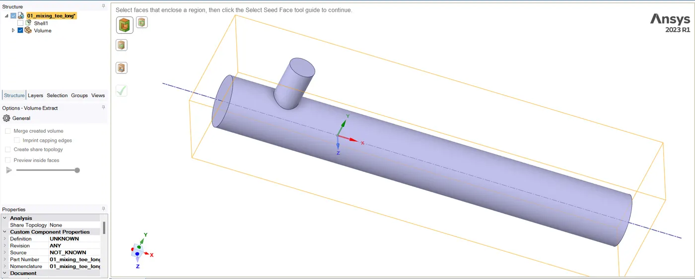
Case 2:
Long Tee mixing:
------------------------------------------------------------------------------------------------------------------------------------
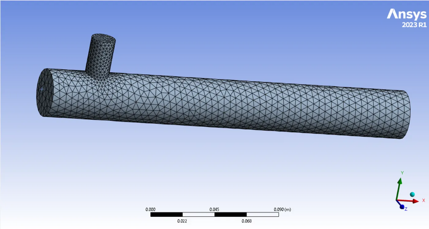
Default Mesh:
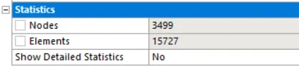
Mesh size: 13.853 mm
Case II-a
hot Inlet velocity - 3m/s
Momentum ratio - 2
cold inlet velocity=3*2 =6 m/s
Turbulence model: K-Epsilon Relizable model
Mesh size: 13.853 mm
Results:
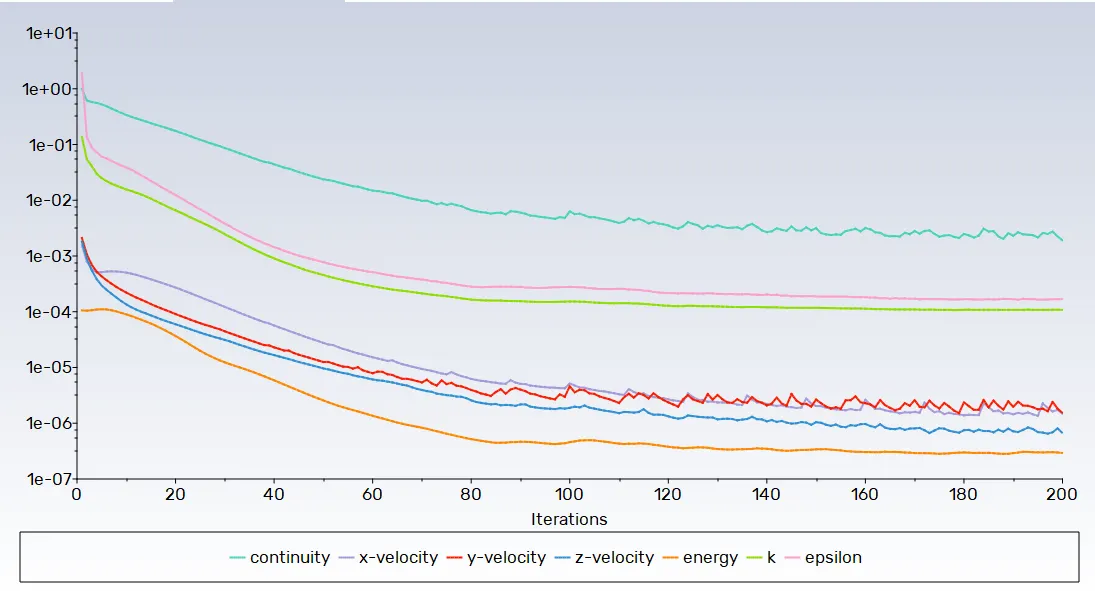
Residual plot:-
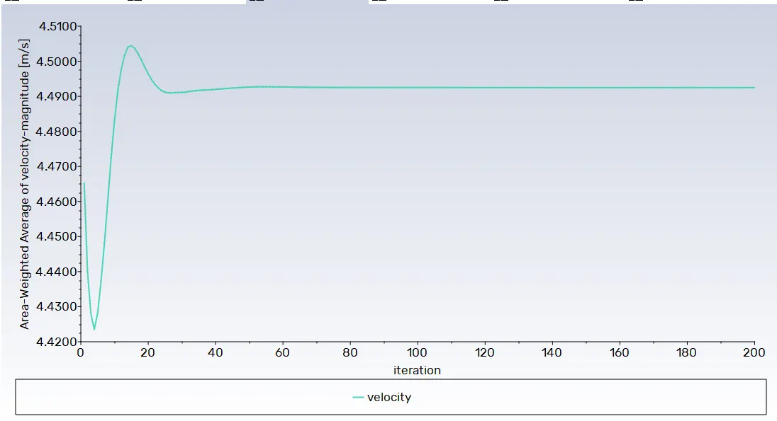
Area weighted average velocity plot:-
Area weighted average temprature plot:-
Standard deviation velocity plot: -
Standard deviation temperature plot: -
Temperature contour plot: -
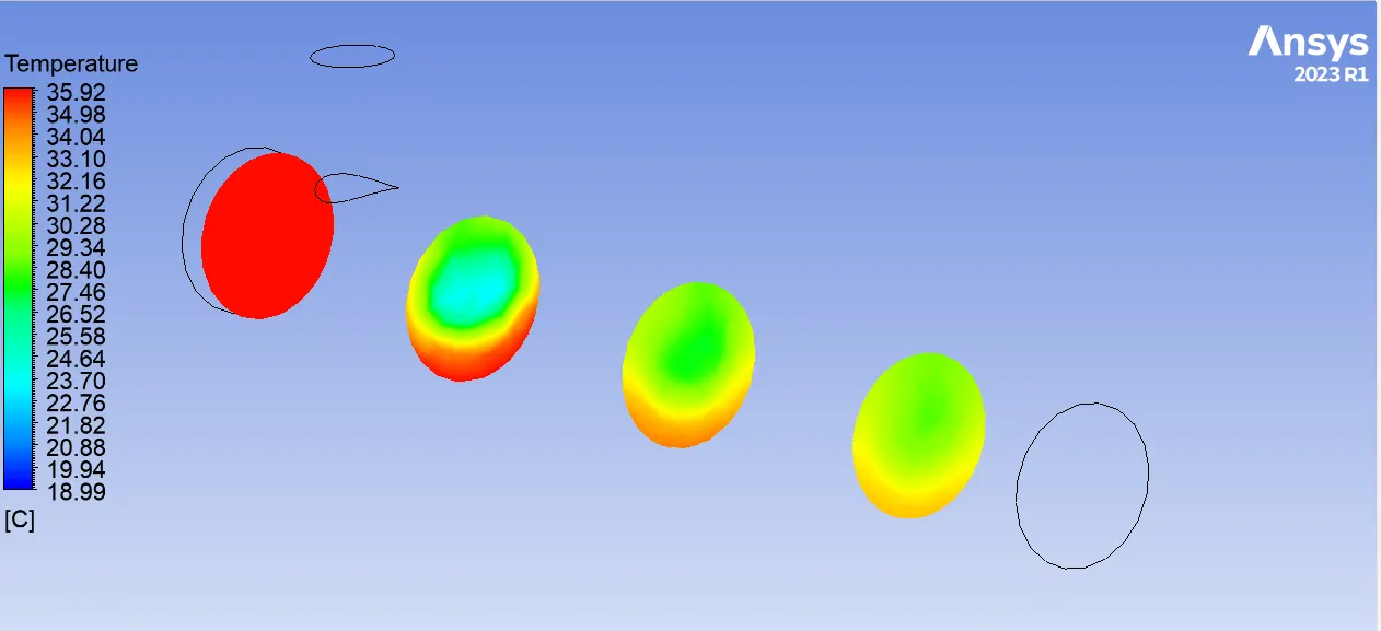
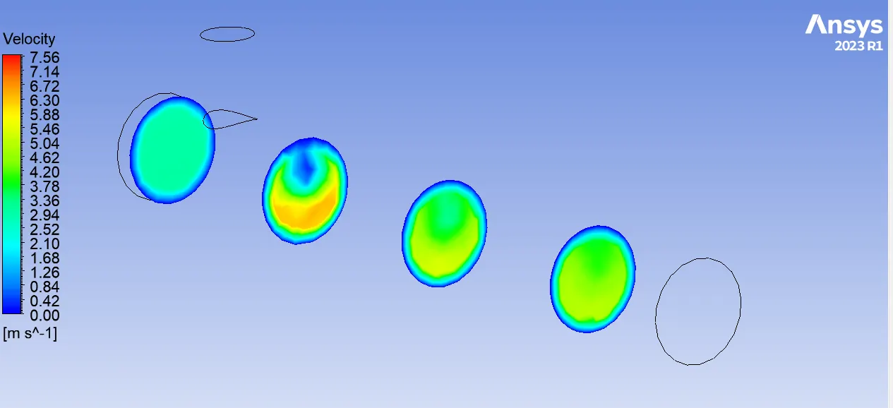
Velocity contour plot:-
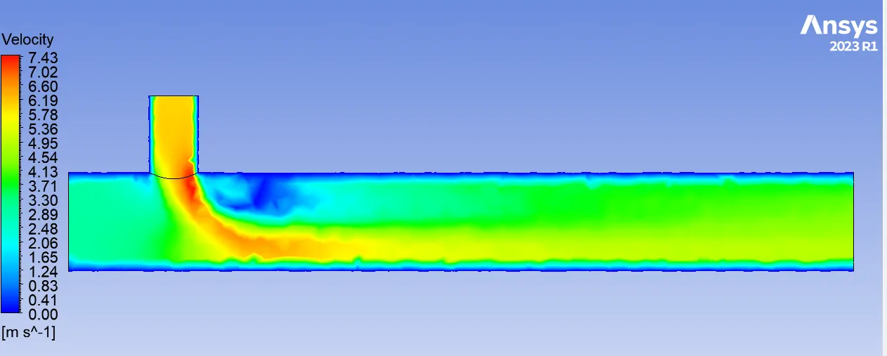
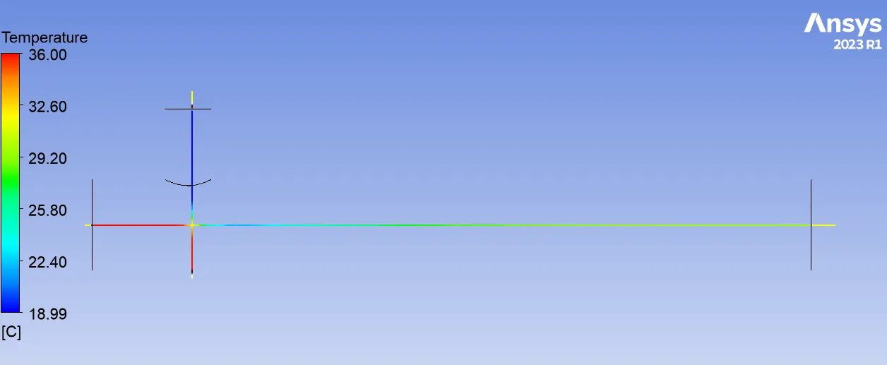
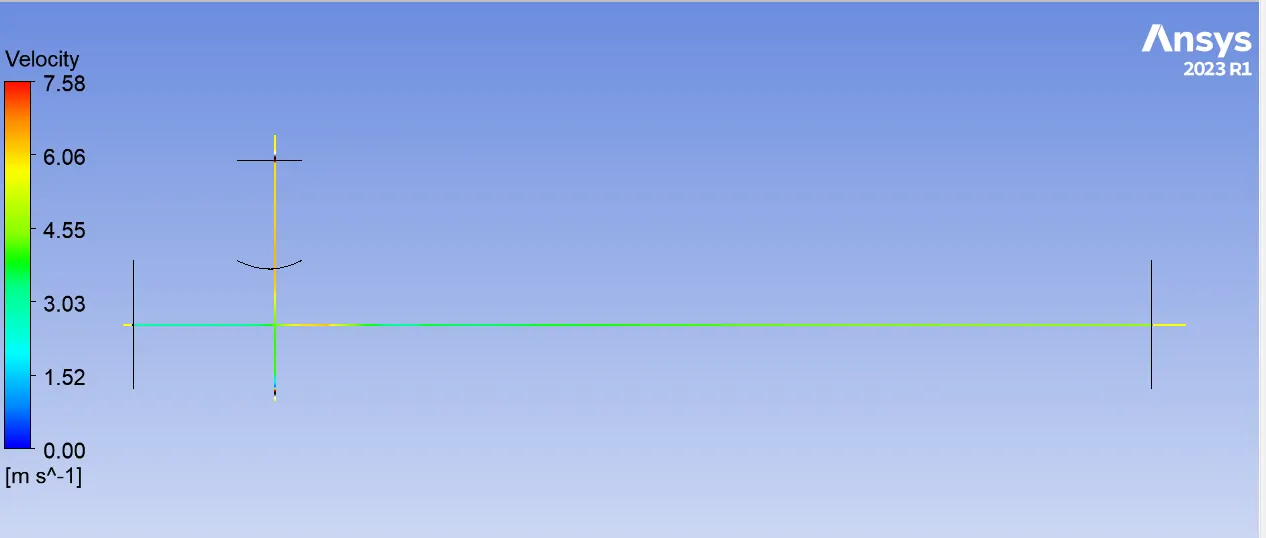
Line Plot:
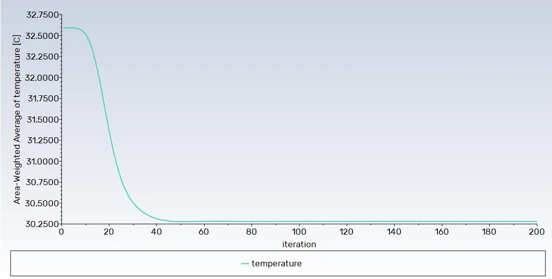
Area Weighted Average velocity at outlet= 4.4924784 m/s
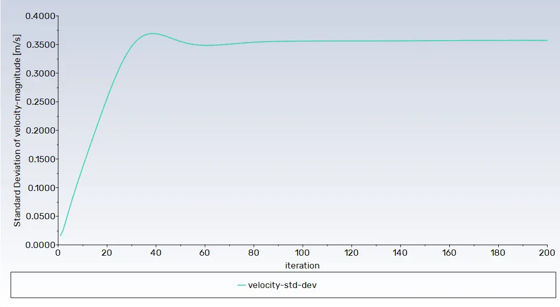
Standard Deviation of velocity at outlet=0.35721943 m/s
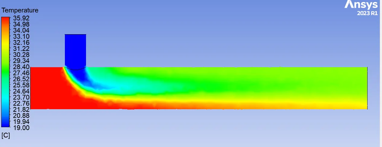
Area Weighted Average Temperature at outlet=30.280436 C
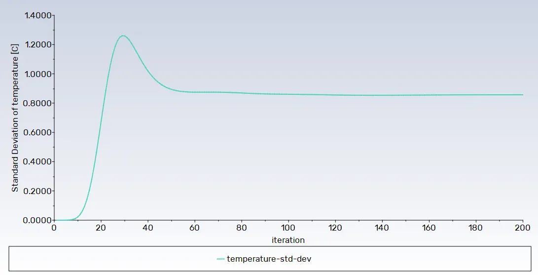
Standard Deviation of temperature at outlet=0.85707357 C
---------------------------------------------------------------------------------------------------------------------------------------
Case-II-b
hot Inlet velocity - 3m/s
Momentum ratio - 4
cold inlet velocity=3*4 =12 m/s
Turbulence model: K-Epsilon Relizable model
Mesh size: 13.853 mm
Results:
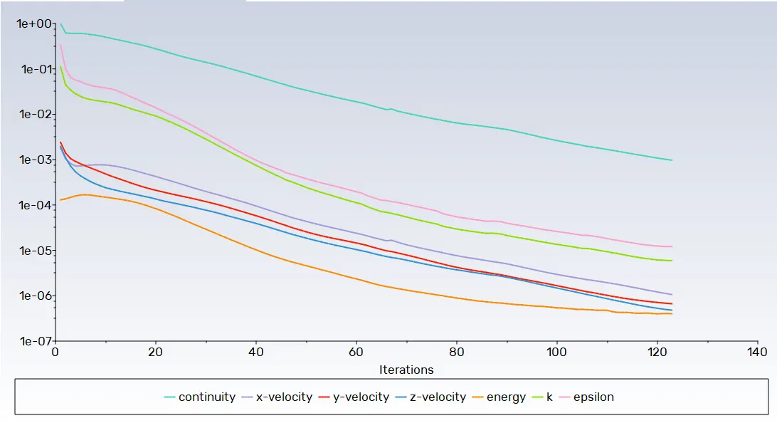
Residual plot:-
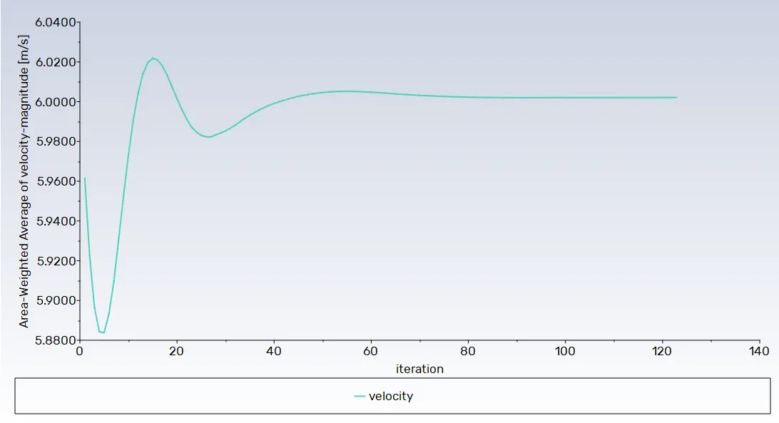
Area weighted average velocity plot:-
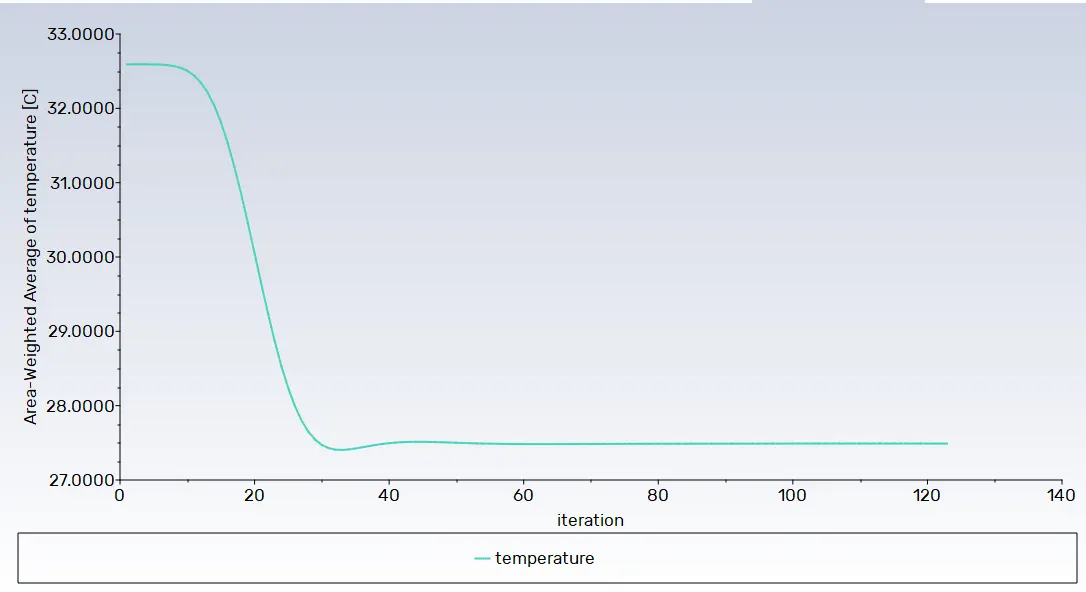
Area weighted average temprature plot:-
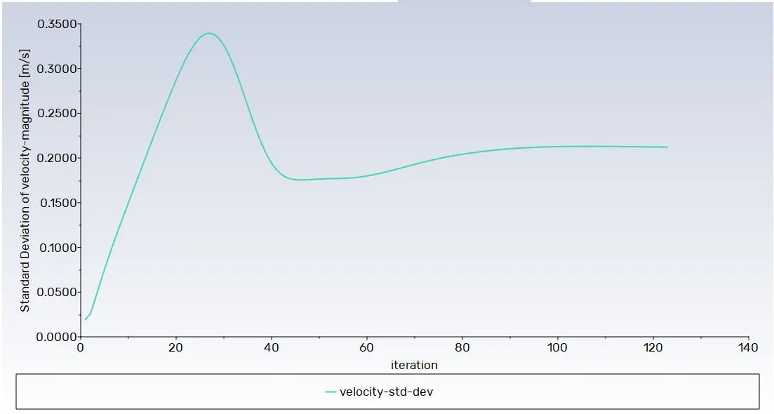
Standard deviation velocity plot: -
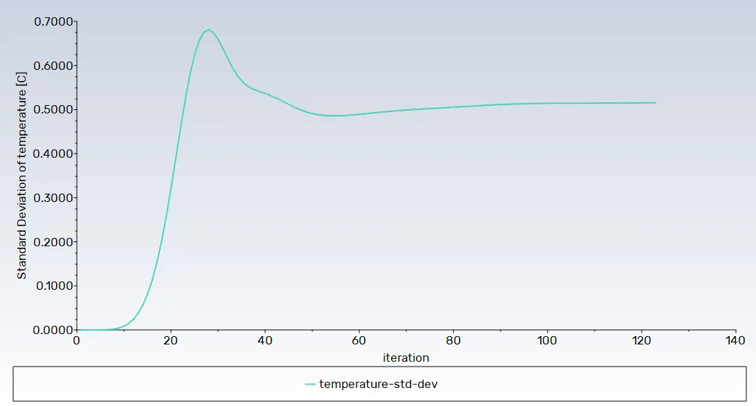
Standard deviation temperature plot: -
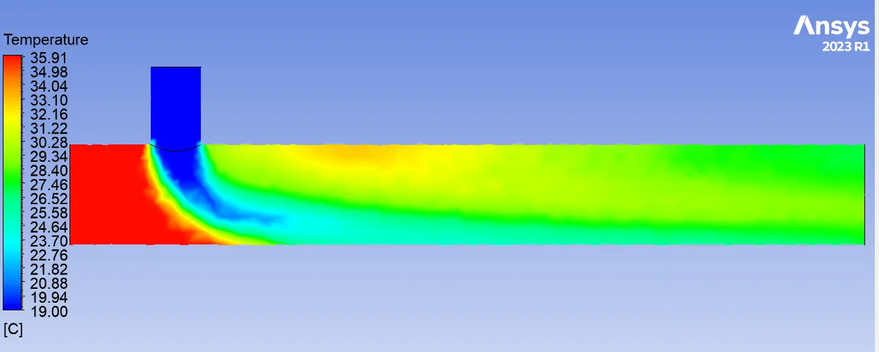
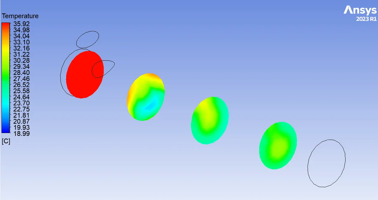
Temperature contour plot: -
Velocity contour plot:-
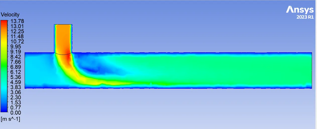
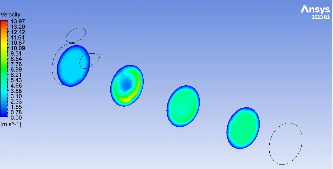
Line Plot:
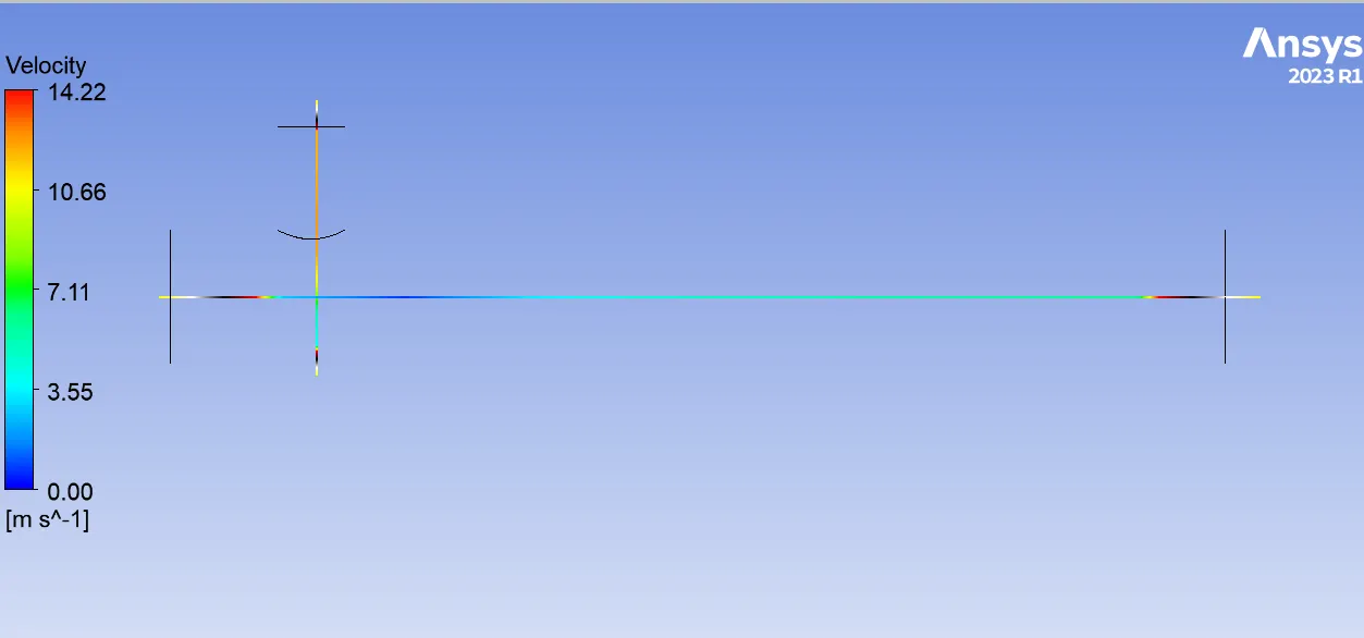
Area Weighted Average velocity at outlet= 6.00421007 m/s
Standard Deviation of velocity at outlet=0.21214452 m/s
Area Weighted Average Temperature at outlet=27.490082 C
Standard Deviation of temperature at outlet=0.51532802 C
------------------------------------------------------------------------------------------------------------------------------------------------------------------------------------------------------------------------------------------------------------------------------
Fine Mesh
Mesh size: 6 mm
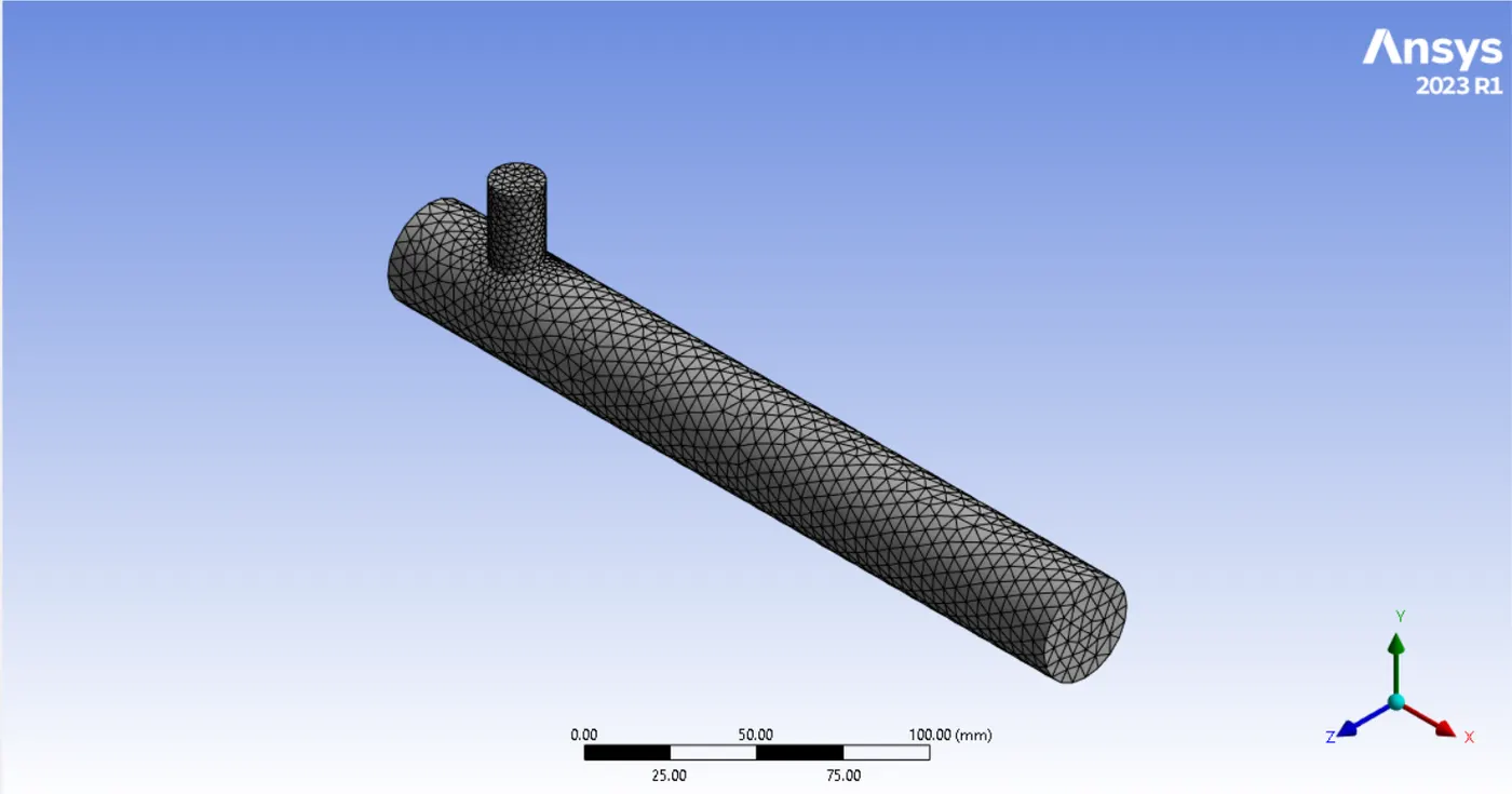

---------------------------------------------------------------------------------------------------------------------------------------
Case II-a
hot Inlet velocity - 3m/s
Momentum ratio - 2
cold inlet velocity=3*2 =6 m/s
Turbulence model: K-Epsilon Relizable model
Mesh size: 6 mm
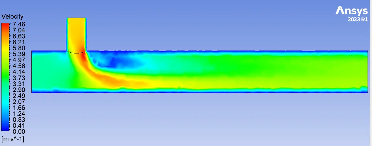
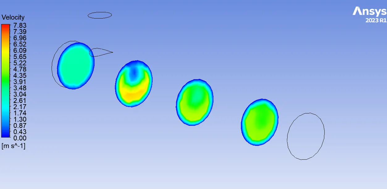
Results:
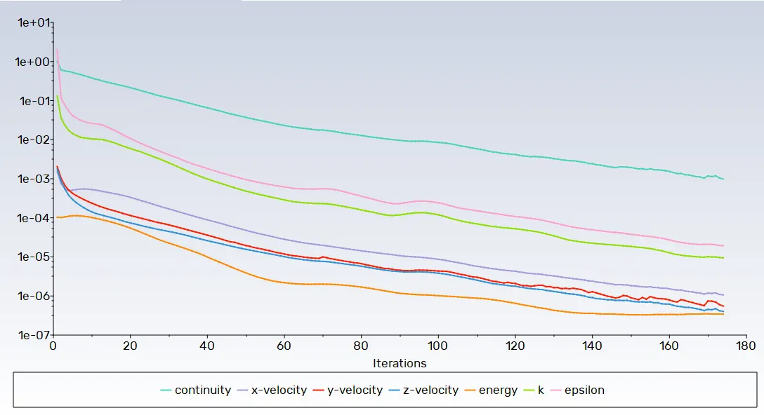
Residual plot:-
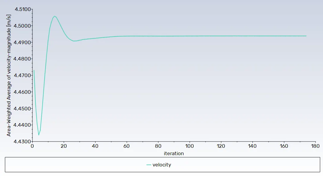
Area weighted average velocity plot:-
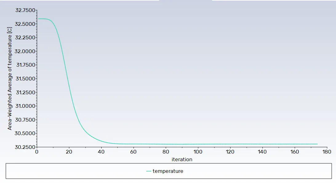
Area weighted average temprature plot:-
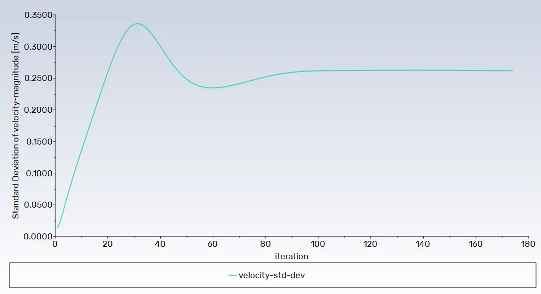
Standard deviation velocity plot: -
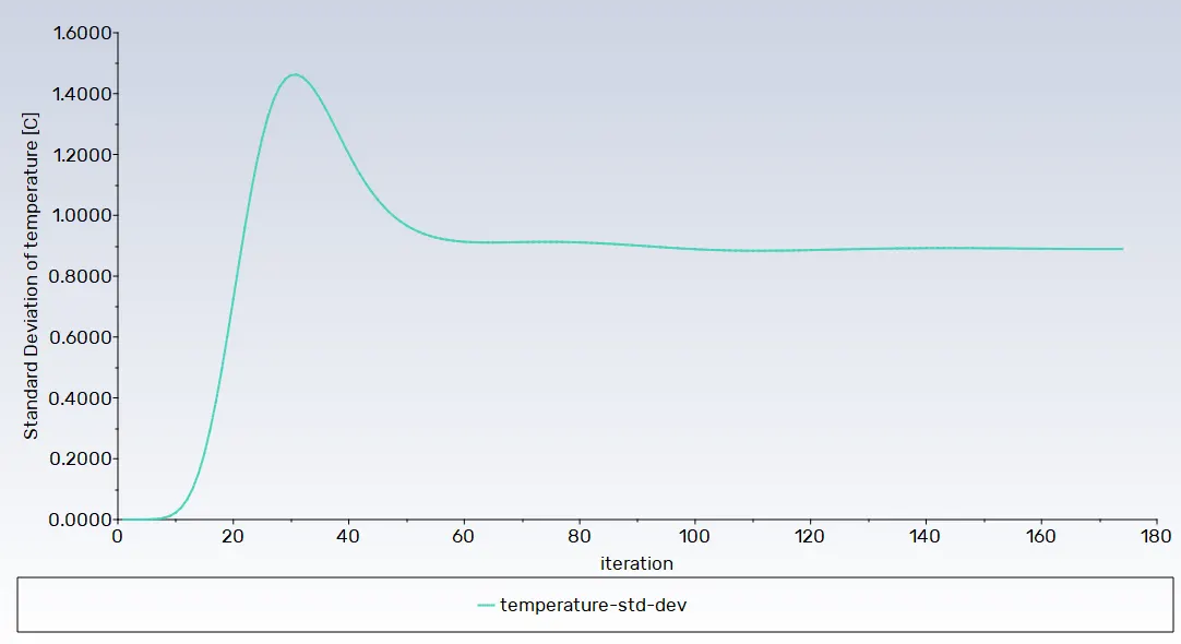
Standard deviation temperature plot: -
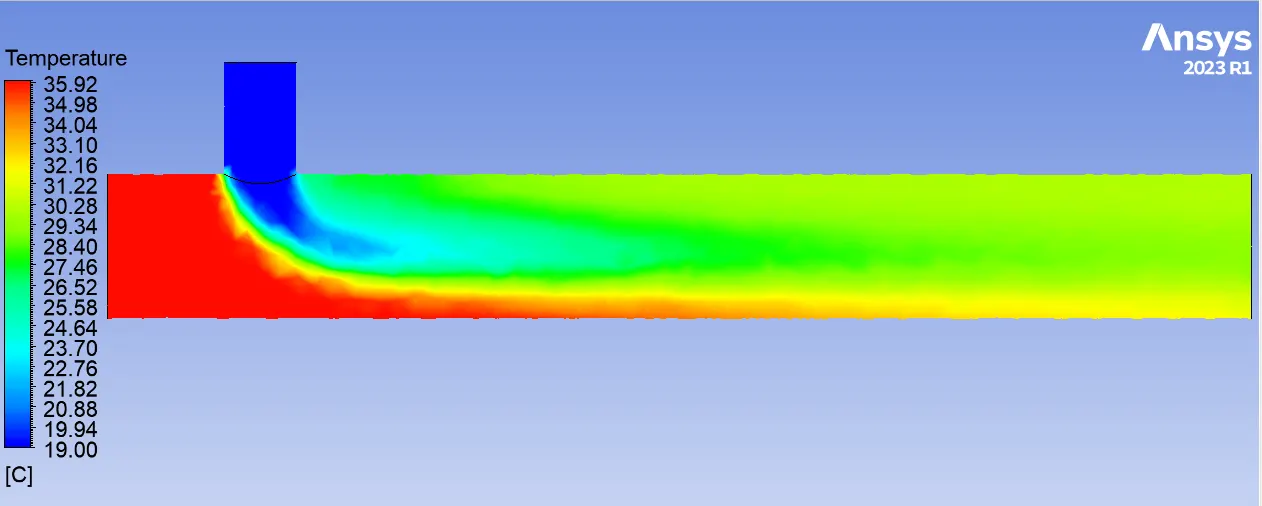
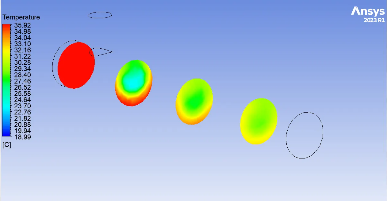
Temperature contour plot: -
Velocity contour plot:-
Line Plot:
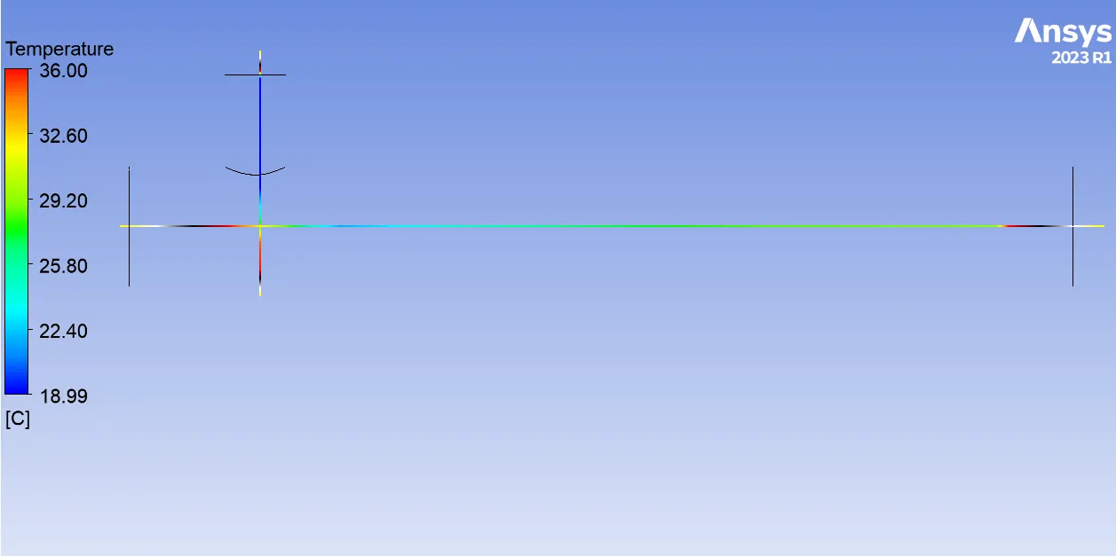
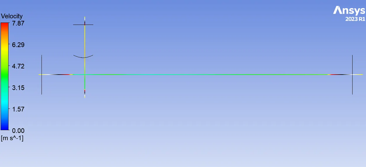
Area Weighted Average velocity at outlet= 4.4938311 m/s
Standard Deviation of velocity at outlet=0.26183445 m/s
Area Weighted Average Temperature at outlet=30.305174 C
Standard Deviation of temperature at outlet=0.88923811 C
--------------------------------------------------------------------------------------------------------------------------------------
Case II -b
hot Inlet velocity - 3m/s
Momentum ratio - 4
cold inlet velocity=3*4 =12 m/s
Turbulence model: K-Epsilon Relizable model
Mesh size: 6 mm
Results:
Residual plot:-
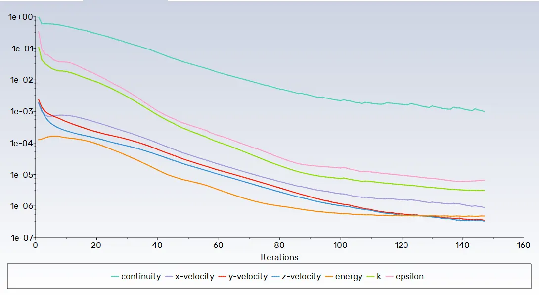
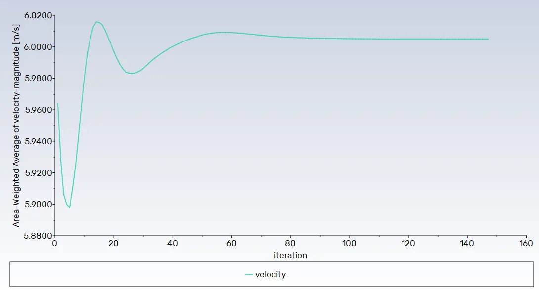
Area weighted average velocity plot:-
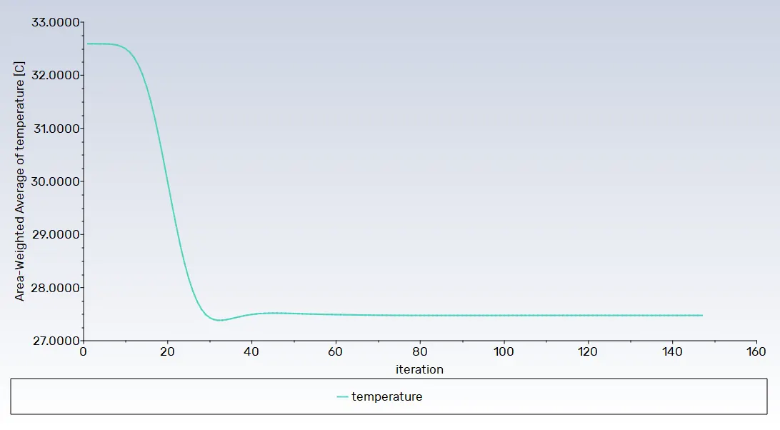
Area weighted average temprature plot:-
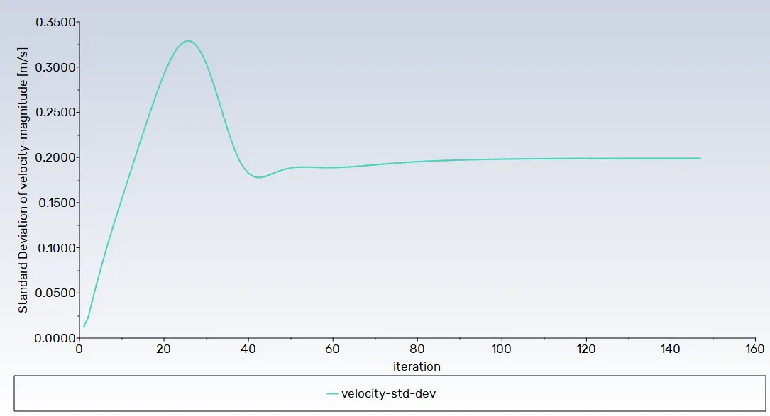
Standard deviation velocity plot: -
Standard deviation temperature plot: -
Temperature contour plot: -
Velocity contour plot:-
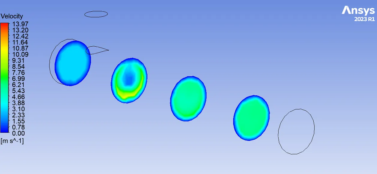
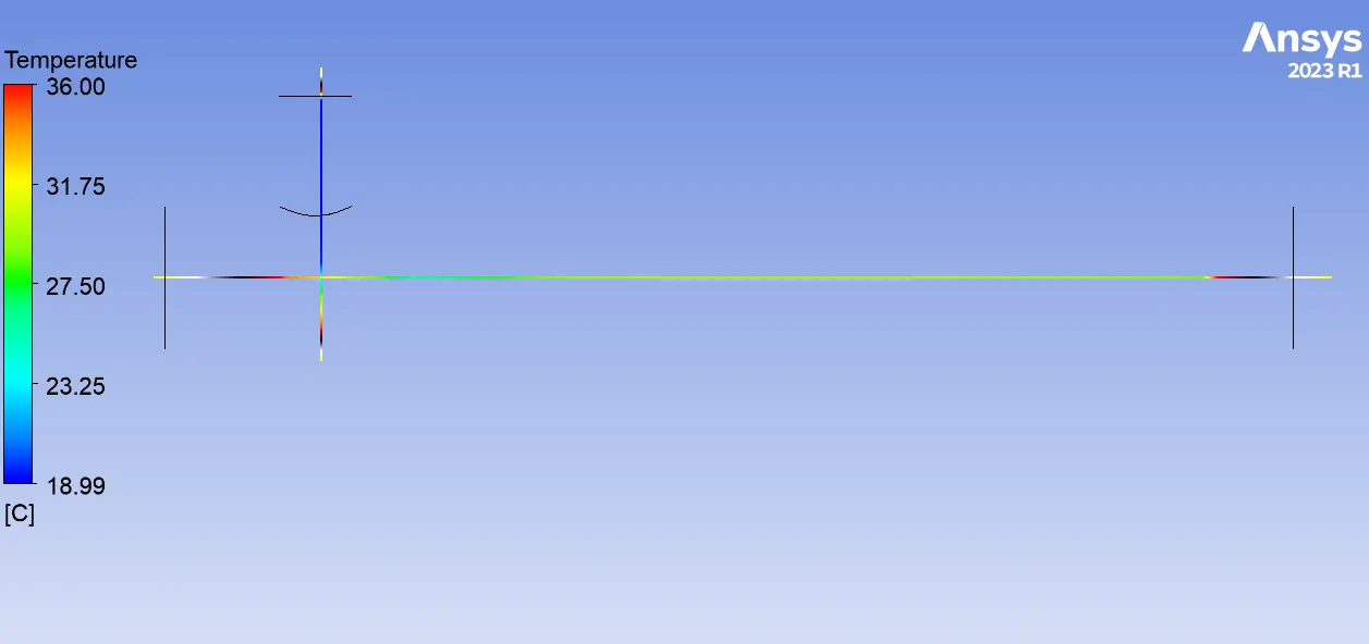
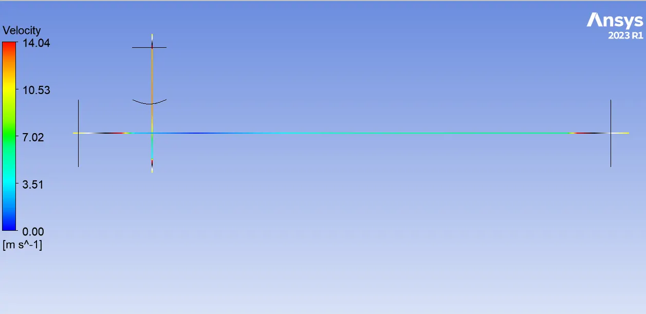
Line Graph:
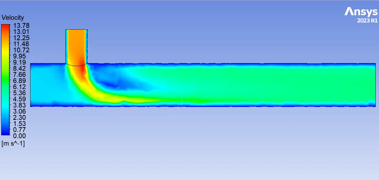
Area Weighted Average velocity at outlet= 6.0049856 m/s
Standard Deviation of velocity at outlet=0.19893743 m/s
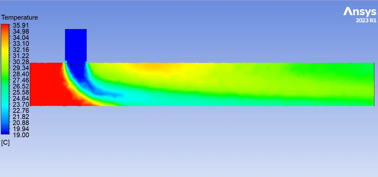
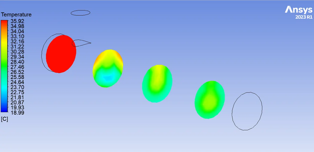
Area Weighted Average Temperature at outlet=27.476528 C
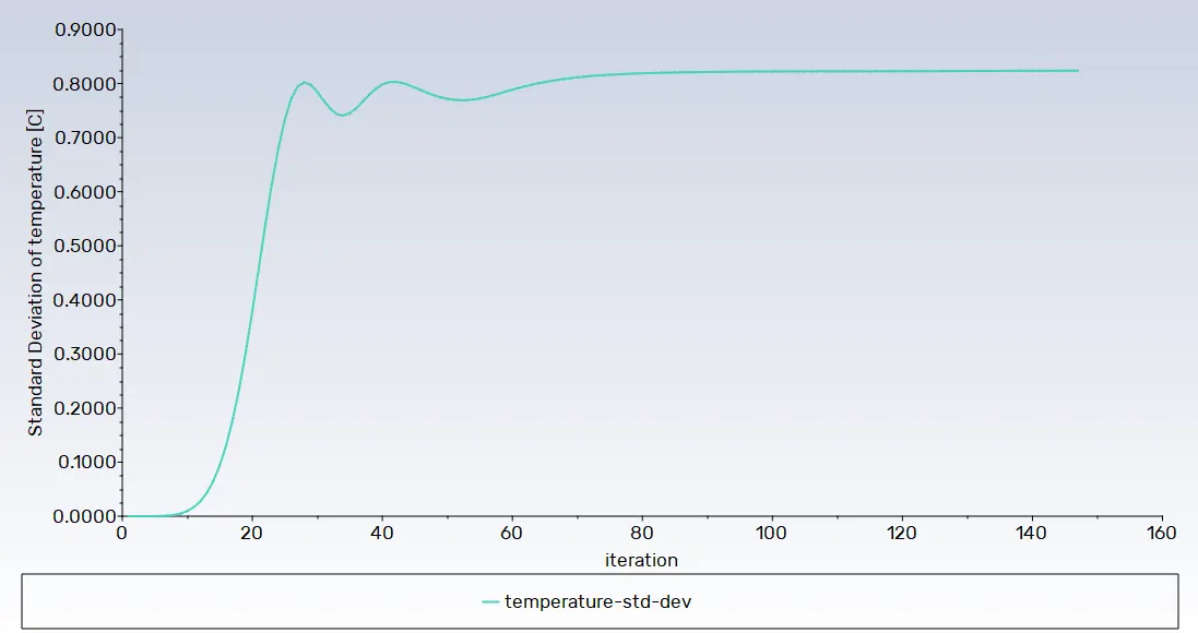
Standard Deviation of temperature at outlet=0.82388859 C
------------------------------------------------------------------------------------------------------------------------------------------------------------------------------------------------------------------------------------------------------------------------------
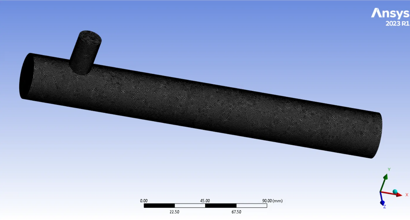
Fine Mesh
Mesh size: 1 mm
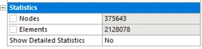
---------------------------------------------------------------------------------------------------------------------------------------
Case II-a
Hot Inlet velocity - 3m/s
Momentum ratio - 2
cold inlet velocity=3*2 =6 m/s
Turbulence model: K-Epsilon Relizable model
Mesh size: 1 mm
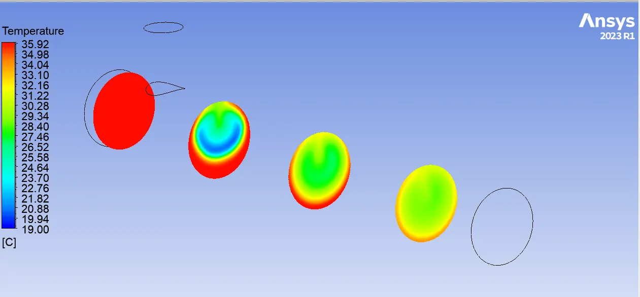
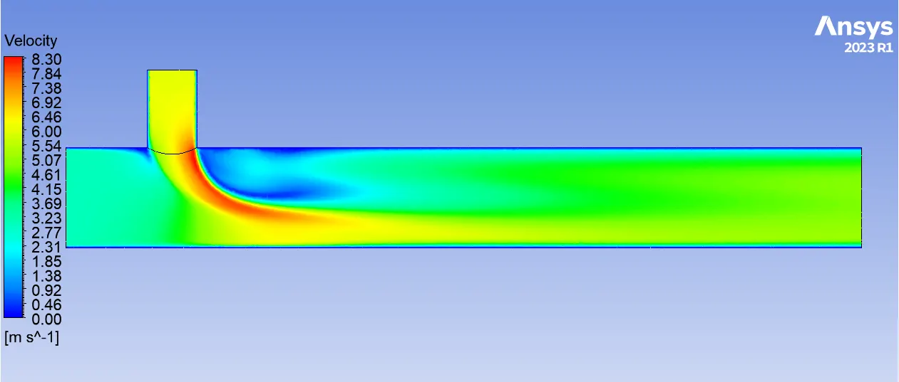
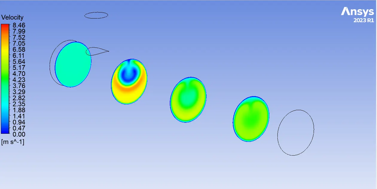
Results:
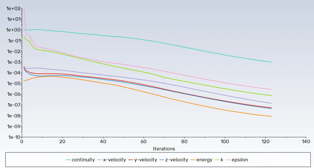
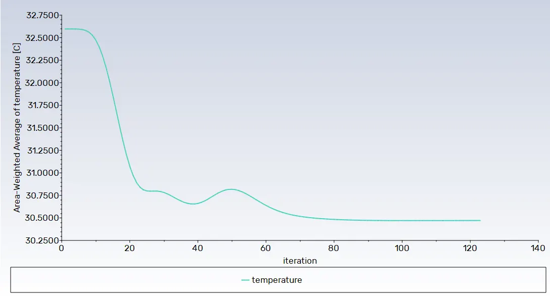
Residual plot:-
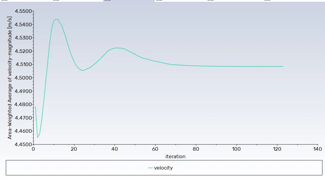
Area weighted average velocity plot:-
Area weighted average temprature plot:-
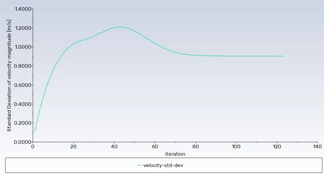
Standard deviation velocity plot: -
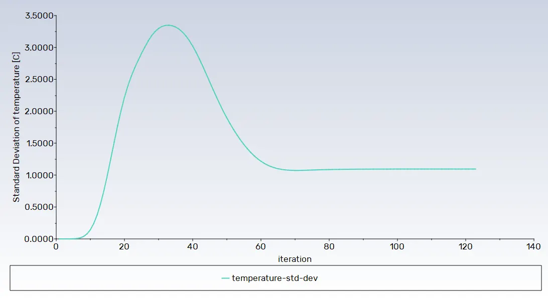
Standard deviation temperature plot: -
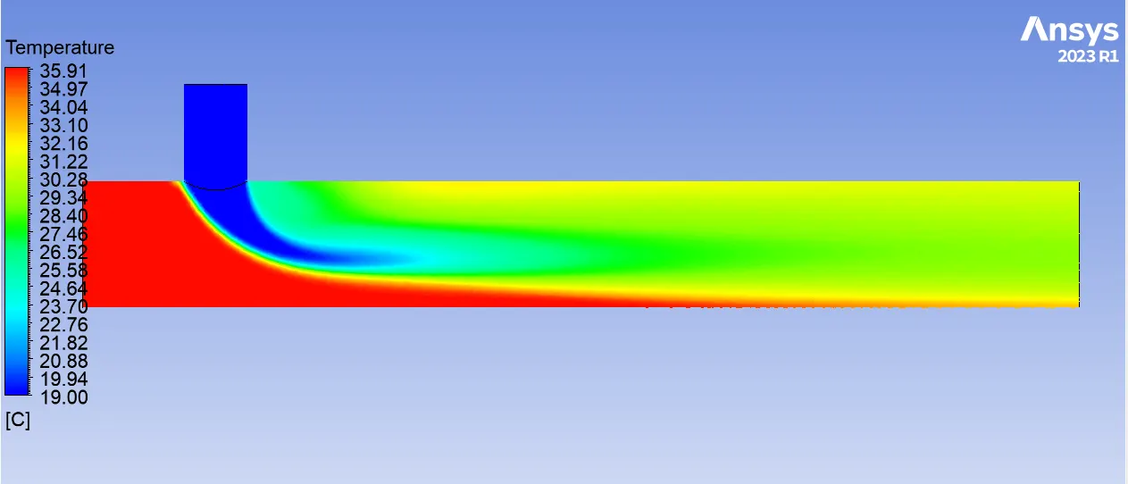
Temperature contour plot: -
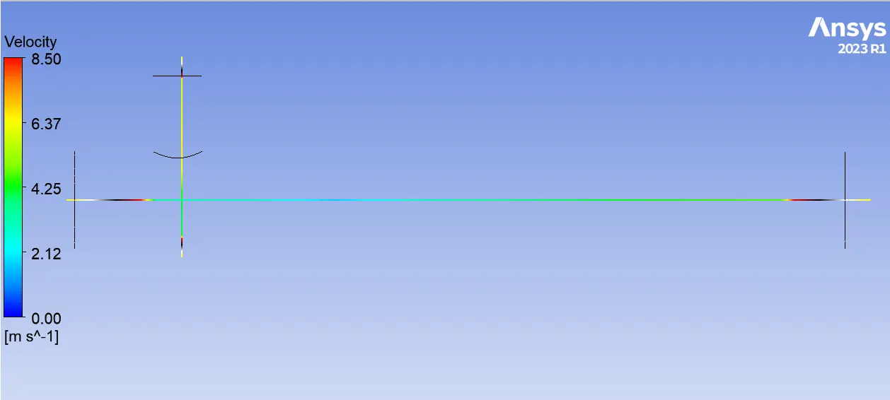
Velocity contour plot:-
Line Plot:
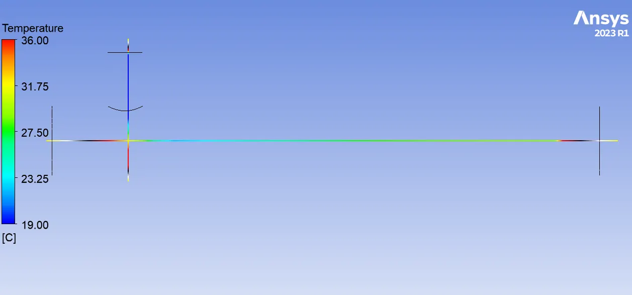
Area Weighted Average velocity at outlet= 4.5049258 m/s
Standard Deviation of velocity at outlet=0.90399087 m/s
Area Weighted Average Temperature at outlet=30.357497 C
Standard Deviation of temperature at outlet=1.0944431 C
---------------------------------------------------------------------------------------------------------------------------------------
Case II -b
Hot Inlet velocity - 3m/s
Momentum ratio - 4
cold inlet velocity=3*4 =12 m/s
Turbulence model: K-Epsilon Relizable model
Mesh size: 1 mm
Results:
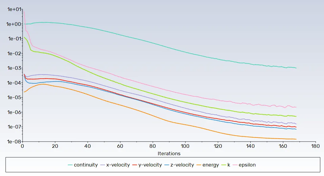
Residual plot:-
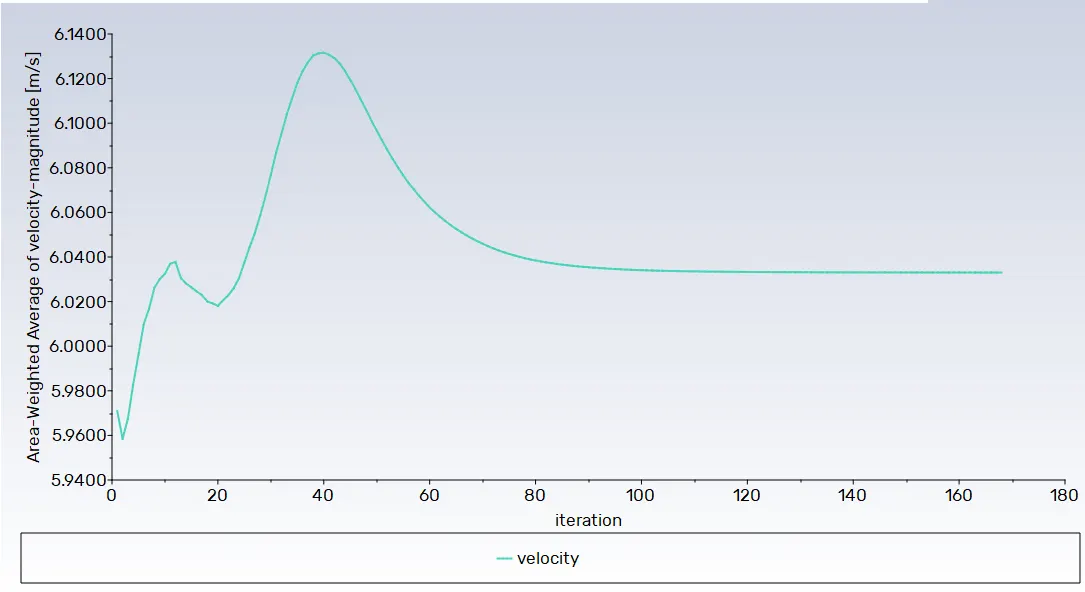
Area weighted average velocity plot:-
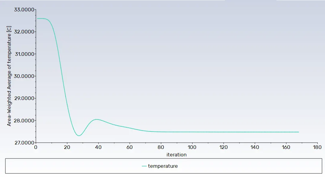
Area weighted average temprature plot:-
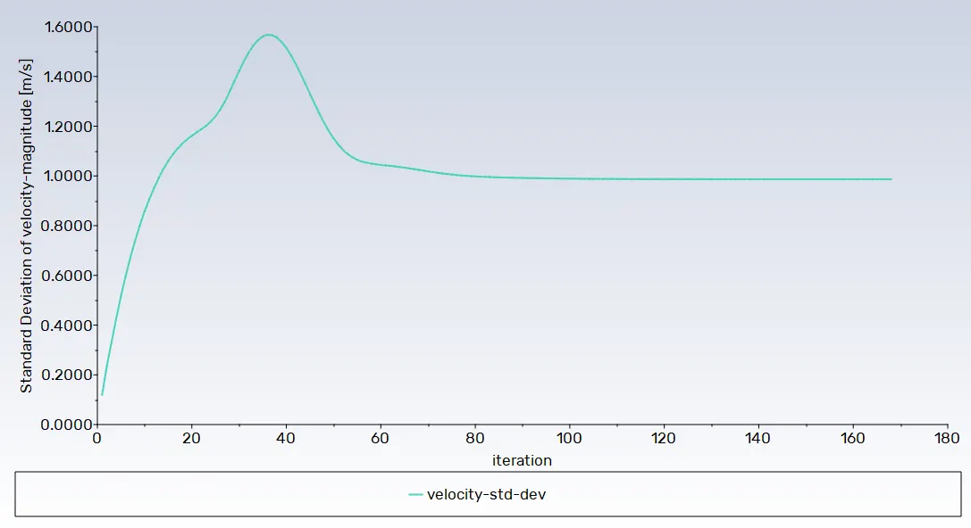
Standard deviation velocity plot: -
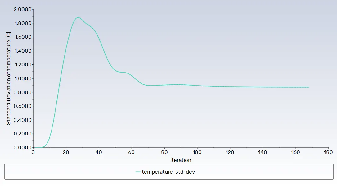
Standard deviation temperature plot: -
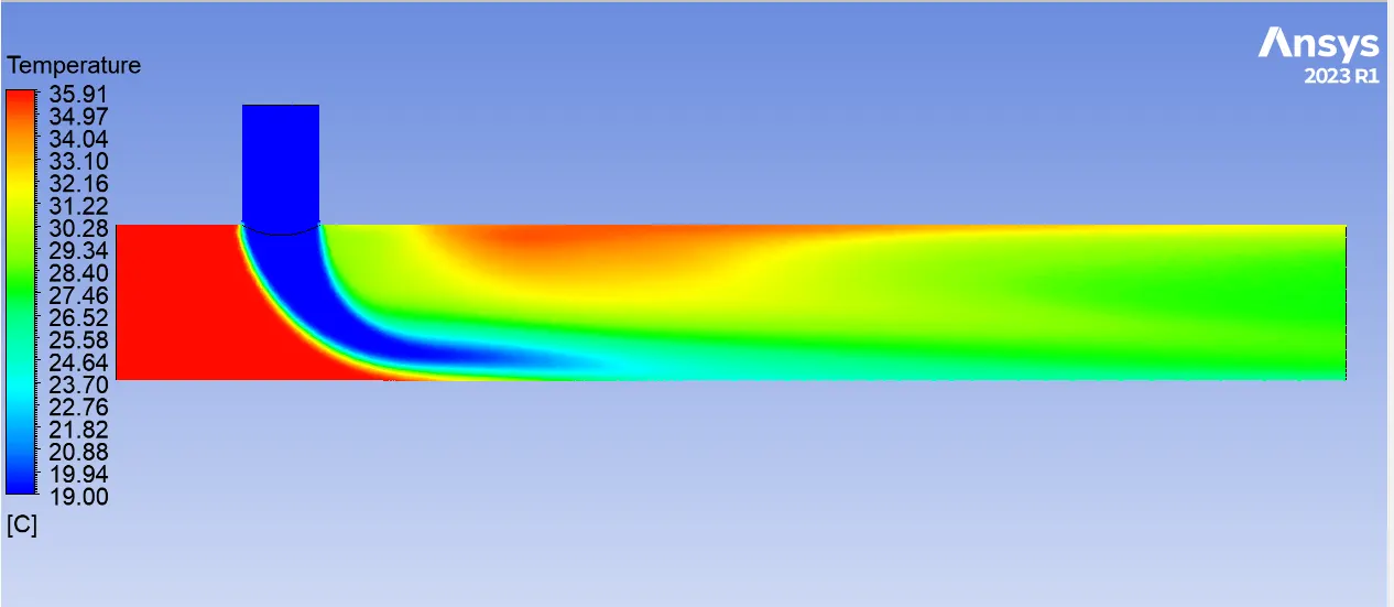
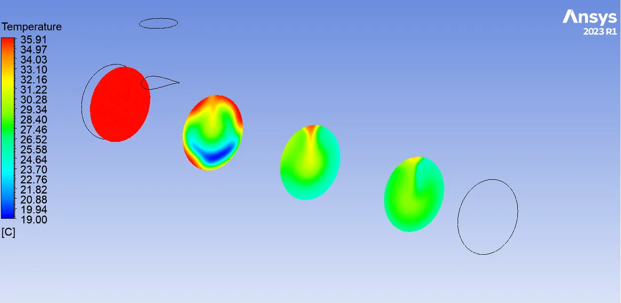
Temperature contour plot: -
Velocity contour plot:-
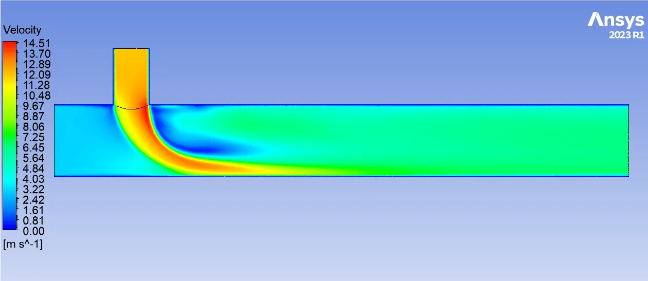
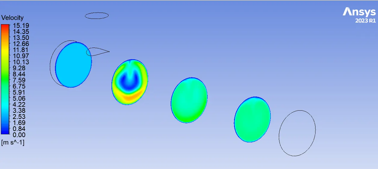
Line Plot:
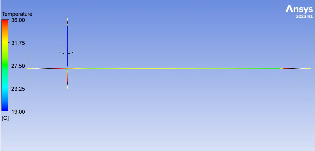
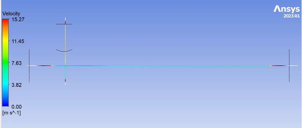
Area Weighted Average velocity at outlet= 6.0330373 m/s
Standard Deviation of velocity at outlet=0.98675212 m/s
Area Weighted Average Temperature at outlet=27.478699 C
Standard Deviation of temperature at outlet=0.87164052 C.
------------------------------------------------------------------------------------------------------------------------------------------------------------------------------------------------------------------------------------------------------------------------------
Project Schematics:
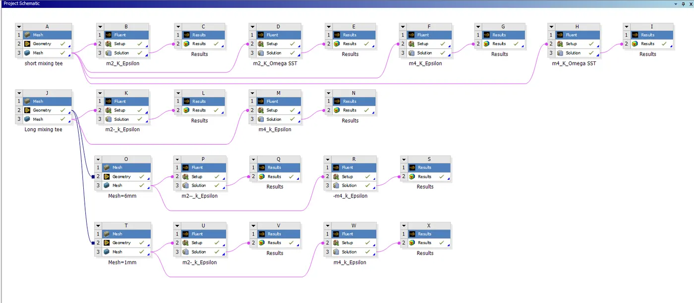
----------------------------------------------------------------------------------------------------------------------------------------------------------------------------------------------------------------------------------------------------------------
ANALYTICAL SOLUTION:
Cold inlet : Hot Inlet:
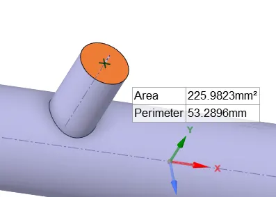
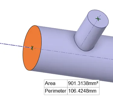
MOMENTUM RATIO 2:
Mass of hot fluid (`m_h`) = `rho**a**V_h` = `997**0.000901**3` = 2.6919 kg/s
Mass of cold fluid (`m_c`) = `rho**a**V_c` = `997**0.000226**6` = 1.351932 kg/s
Temperature of mixture (Tmixture) = `(m_h**T_h + m_c**T_c)/(m_c + m_h)` = 30.3207 C
MOMENTUM RATIO 4:
Mass of hot fluid (`m_h`) = `rho**a**V_h` = `997**0.000901**3 `= 2.6919 kg/s
Mass of cold fluid (`m_c`) = `rho**a**V_c` = `997**0.000226**12` = 2.703864 kg/s
Temperature of mixture (Tmixture) = `(m_h**T_h + m_c**T_c)/(m_c + m_h)` = 27.48 C
Comparison Table:
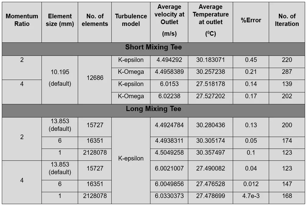
- Upon consolidating the findings into a comprehensive table, comparison reveals that the output results are minimally influenced by the length of the mixing tee, particularly when disregarding the diffusion criteria.
- High-velocity flow showing good mixing results than low-velocity flow.
- All results are passing the mesh independence criteria.
CONCLUSION:
- Independence of Output Temperature on Mixing Tee Length: Results from both cases indicate that the output temperature is not influenced by the length of the mixing tee.
- Increasing the momentum ratio leads to a sudden drop in the outlet temperature.
- k-epsilon models predict flow away from the wall, while k-omega models predict near the wall. For this case requiring turbulent flow simulation away from the wall, the k-epsilon method is utilized.
- Mesh Quality and Convergence:
Initial simulation on a coarse mesh provides a quick overview and fast convergence of results. - Increasing the element number prolongs convergence time.
- Starting with a coarse mesh allows for efficient improvement of mesh quality, saving time and aiding in achieving accurate final results. This step is particularly valuable for mesh independence testing.
- Higher flow velocity at the outlet significantly improves mixing, emphasizing the effectiveness of a high momentum ratio.
- Diffusion flow in longer mixing tees tends to yield slightly better mixing of the two fluids.
- Optimal Conditions for Precise Results:
-Use a short mixing tee with a momentum ratio of 4.
-Consider the diffusion of flow along the length of the mixing tee.
-A longer mixing tee with a higher momentum ratio can be a favorable option.