Week 11 - Simulation of Flow through a pipe in OpenFoam

AIM:

The aim of this study is to simulate an axi-symmetric flow within a constant cross-section pipe by implementing a wedge boundary condition.

OBJECTIVES:

The primary objectives of this project are as follows:

• Simulate an axi-symmetric flow within a constant cross-section pipe at an inlet Reynolds number of 2100 while applying a wedge boundary condition.
• Conduct a transient or steady-state simulation to validate the results with the Hagen-Poiseuille equations for fully developed flow.
• Develop a MATLAB code to automate the simulation of an axi-symmetric flow in openfoam.
• To obtain the following results from the simulation:

i. Validate the hydrodynamic length with numerical results.

ii. Validate the fully developed flow velocity profile against its analytical counterpart.

iii. Validate the maximum velocity and pressure drop for fully developed flow.

iv. Post-process shear stress and validate wall shear stress for fully developed flow.

The problem at hand involves creating a wedge from a hexagonal block by merging its bottom face through collapsing, resulting in a wedge angle less than 5 degrees. The pipe diameter can be assumed.

INTRODUCTION:

Flow-through pipes, or fluid flow within closed conduits, entails a particular pressure-driven flow of real fluids, which exhibit viscosity. Viscous flows are characteristic of real fluids, where viscosity is the property responsible for shear stresses and frictional forces between fluid layers and solid surfaces.

THEORY:

Axisymmetric Flow

Axisymmetric flow is a type of flow in which flow variables, such as velocity and pressure, remain constant with respect to the angular coordinate θ. To address computational limitations, this study employs an axi-symmetric approach to simulate a section of a cylinder, known as a wedge, rather than the entire domain. This approach leverages the axisymmetric nature of the flow, applying a symmetry boundary condition to reduce computational demands.

Laminar Flow:

Laminar flow is a well-ordered and highly organized type of flow where fluid streamlines are smooth, parallel, and free from disruptive mixing. At low velocities, fluid particles move in an orderly fashion, sliding past one another without significant lateral dispersion. This type of flow lacks cross-currents, eddies, or turbulent swirls. In laminar flow, particles within the fluid follow predictable paths, moving in straight lines parallel to the pipe walls. This behavior results in a coherent and regular flow pattern.

Turbulent Flow:

Conversely, turbulent flow is characterized by irregular and chaotic fluid motion. In turbulent flow, streamlines are not smooth, and velocity fluctuations occur in a highly disordered manner. This flow regime is marked by rapid and unpredictable changes in pressure and velocity over time and space. Unlike laminar flow, there is no distinct layering of fluid, and mixing within the pipe is highly efficient. As fluid moves through a turbulent flow regime, it experiences continuous fluctuations and irregularities.

Example:

Oil Pipelines: Flow in oil pipelines can transition from laminar to turbulent when there are changes in pipeline diameter, bends, or the introduction of pumps. This transition can influence energy requirements and the maintenance of pipelines.

Reynolds Number:

The Reynolds number (Re) is a fundamental parameter in fluid mechanics that determines whether a flow condition is laminar or turbulent. It is defined as the ratio of inertial forces to viscous forces within a fluid. The Reynolds number is calculated using the following formula:

`Re = (rho * V * D) / mu`

Where:

- `rho` is the density of the fluid (kg/m³)

- V is the velocity of the fluid (m/s)

- D is a characteristic length (m)

- `mu` is the dynamic viscosity of the fluid (Pa·s or N·s/`m^2` or kg/(m·s))

The critical Reynolds number (`Re_{cr}`) indicates the point at which a flow becomes turbulent. For internal flow in a circular pipe, `Re_{cr}` is typically accepted as 2300. Under most practical conditions:

- Flow is laminar for Re ≲ 2300

- Flow is turbulent for Re ≳ 4000

- Transitional flow occurs in between (2300 ≲ Re ≲ 4000)

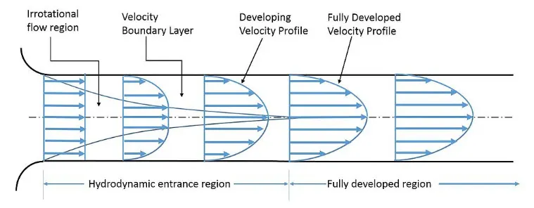
Fully Developed Flow

Fully developed flow is characterized by the establishment of a complete velocity profile within the pipe, where viscous effects due to shear stress between fluid particles and the pipe walls have reached equilibrium. The region from the pipe inlet to the point of a fully developed velocity profile is referred to as the hydrodynamic entrance region. Flow within the entrance region is known as hydrodynamically fully developed flow since this is where the velocity profile matures.

Entrance Length:

The entrance length refers to the distance a fluid travels within a pipe before it achieves a fully developed flow state. This length encompasses the entry region following the pipe entrance, where effects originating from the interior pipe wall propagate into the flow as an expanding boundary layer. Once the boundary layer expands to occupy the entire pipe, the developing flow becomes fully developed, where flow characteristics remain constant along the pipe's length.

The hydrodynamic entry length is commonly defined as the distance from the pipe entrance to where the wall shear stress reaches approximately 2 percent of its fully developed value. In laminar flow, the nondimensional hydrodynamic entry length is approximated as:

`L_(laminar)/D ≅ 0.05 * Re`

For turbulent flow, the intense mixing during random fluctuations usually overshadows the effects of molecular diffusion, and the nondimensional hydrodynamic entry length is approximated as:

`L_(turbulent)/D = 1.359 * (Re)^{1/4}`

Velocity Profile for Laminar Flow through a Circular Pipe:

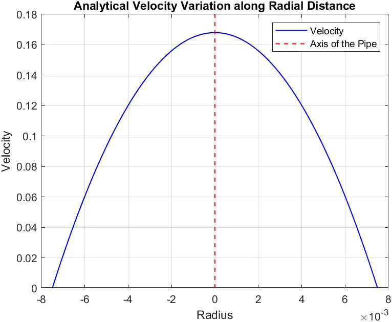
In fully developed laminar flow through a straight circular pipe, the velocity profile is parabolic. This profile exhibits a maximum velocity at the centerline and decreases to zero at the pipe wall. The velocity profile is expressed as:

`U(r) = 2 * V_{avg}* (1 - (r^2 / R^2))`

Where:

- U(r) is the velocity at a radial distance r from the pipe centerline.

- `V_{avg}` is the average velocity.

- R is the pipe radius.

The maximum velocity (Umax) occurs at the centerline (r = 0) and is equal to 2 times the average velocity.

Pressure Drop:

The pressure drop (ΔP) in pipe flow is a significant parameter related to the power requirements for maintaining flow. It is represented as:

`gradP = 8 * mu * L * V_{avg} / R^2`

Where:

- `mu` is the fluid viscosity.

- L is the length of the pipe (beyond the entry length).

-`V_{avg}` is the average velocity.

- R is the pipe radius

Hagen-Poiseuille's Theory

The Hagen-Poiseuille equation, or the Poiseuille law, describes pressure drop in incompressible and Newtonian fluids in laminar flow through long cylindrical pipes. This equation applies to flows in pipes with constant circular cross-sections that are substantially longer than their diameter and where there is no fluid acceleration. The Hagen-Poiseuille equation is given by:

`ΔP = 32 * mu * L * V_{avg} / D^2`

Where:

- `mu` is the fluid viscosity.

- L is the length of the pipe (beyond the entry length).

- `V_{avg}` is the average velocity.

- D is the diameter of the pipe.

This equation relates pressure drop, fluidic resistance, and flow rate, much like Ohm's law for electrical circuits (V=RI). To apply the Hagen-Poiseuille equation effectively, the ratio of pipe length to radius should be greater than one forty-eighth of the Reynolds number.

The Hagen-Poiseuille law finds practical application in various scenarios, such as analyzing air flow in lung alveoli, fluid flow through a drinking straw, or blood flow through narrow constrictions.

METHODOLOGY:

For the numerical simulation conducted in the OpenFOAM software, an axisymmetric wedge domain was employed, and appropriate boundary conditions were applied to achieve accurate flow simulation while minimizing assumptions. This methodology aimed to emulate real-world fluid flow dynamics in a controlled environment.

Lets consider the below image as reference to construct the wedge:

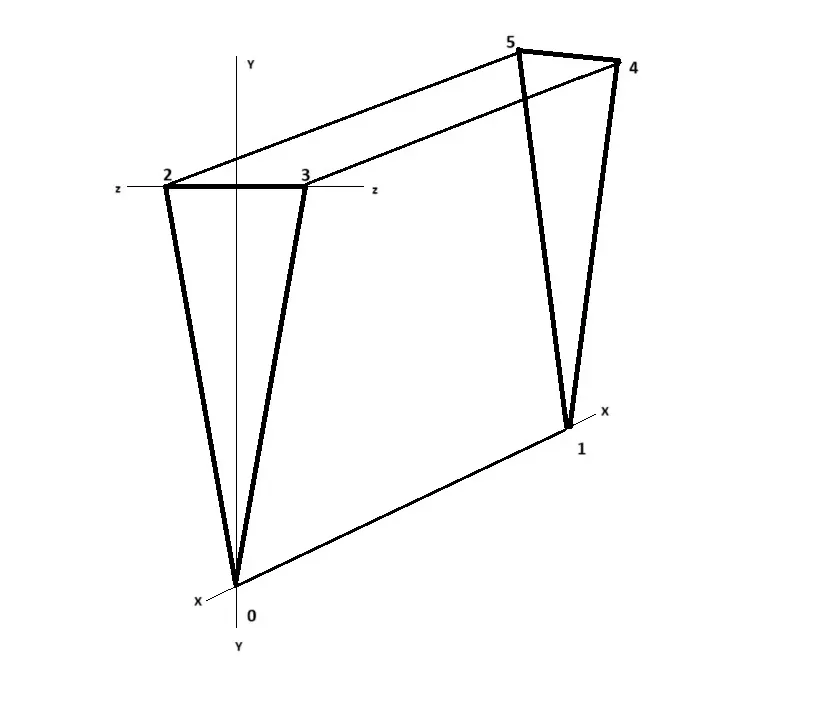
If the wedge length is 'Lpipe' and angle is 'theta'

then,

Diameter of the pipe in meters, d=0.015

Radius, r = d / 2

Angle of wedge, theta = 4.5

Length of developing flow, Lhydro = 0.05 * Re * d=1.5750 m

Length of pipe, Lpipe = Lhydro + 0.1*Lhydro=1.7325 m

Coordinates of vertices of the wedge:

v0 = [0, 0, 0]

v1 = [Lpipe, 0, 0]

v2 = [0, r * cos(theta / 2), -r * sin(theta / 2)]

v3 = [0, r * cos(theta / 2), r * sin(theta / 2)]

v4 =[ Lpipe, r * cos(theta / 2), r * sin(theta / 2)]

v5 = [Lpipe, r * cos(theta / 2), -r * sin(theta / 2)]

Fluid considered for simulation: PETROL

Properties of Fluid (Petrol)

kinematic viscocity at 40 C , `nu`=0.6e-6 `m^2/s`

Density of petrol, `rho`=756.8 `(kg)/m^3`

PROGRAM:

main code:

% Fluid flow in a pipe (Hagen-Poiseuille flow)
%code to automate generation of files for OPEN-FOAM

clear all
close all
clc

%The Renoylds number
Re=2100;
%Diameter of the pipe in meters
d=0.015;
%radius
r = d / 2;
%length of developing flow
Lhydro = 0.05 * Re * d
%length of pipe
Lpipe = Lhydro + 0.1*Lhydro
%Angle of the wedge in degrees
theta=4.5;
%% properties of Fluid (Petrol) 
%kinematic viscocity (m^2/s) at 40 C
nu=0.6e-6;
%Density in kg/m^3 of petrol 
rho=756.8;
%Dynamic viscosity
mu=nu*rho
%% Haigen poisuelle flow equations
%Avg velocity
V_avg=(Re*mu)/(rho*d)
%Maximum velocity 
Vmax=2*V_avg
%Piezo metric pressure drop 
del_p=32*mu*V_avg*0.158/d^2
%Kinematic pressure 
Kinematic_p=del_p/rho

%% Specifying the inputs for blockmeshdict


% Coordinates of vertices
v0 = [0 0 0];
v3 = [0 r * cosd(theta / 2) r * sind(theta / 2)];
v2 = [0 r * cosd(theta / 2) -r * sind(theta / 2)];
v1 = [Lpipe 0 0];
v4 = [Lpipe r * cosd(theta / 2) r * sind(theta / 2)];
v5 = [Lpipe r * cosd(theta / 2) -r * sind(theta / 2)];

% Number of cells along x, y, and z axis
nx = 30;
ny = 1;
nz = 300;

% Grading factors
gx = 0.2;
gy = 1;
gz = 1;

%% edit parameters for controlDict file
endTime=30;
deltaT=0.05;
writeInterval=10;

%% BLOCKMESHDICT FILE
% Creating the file
% Header
h1 = '/*--------------------------------*- C++ -*----------------------------------*\';
h2 = '  =========                 |';
h3 = '  \\      /  F ield         | OpenFOAM: The Open Source CFD Toolbox';
h4 = '   \\    /   O peration     | Website:  https://openfoam.org';
h5 = '    \\  /    A nd           | Version:  11';
h6 = '     \\/     M anipulation  |';
h7 = '\*---------------------------------------------------------------------------*/';
h8 = 'FoamFile';
h9 = '{';
h10 = '    format      ascii;';
h11 = '    class       dictionary;';
h12 = '    object      blockMeshDict;';
h13 = '}';
h14 = '// * * * * * * * * * * * * * * * * * * * * * * * * * * * * * * * * * * * * * //';


% Creating BlockMesh File
f1 = fopen('blockMeshDict','w');

% Header
fprintf(f1,'%s\n',h1);
fprintf(f1,'%s\n',h2);
fprintf(f1,'%s\n',h3);
fprintf(f1,'%s\n',h4);
fprintf(f1,'%s\n',h5);
fprintf(f1,'%s\n',h6);
fprintf(f1,'%s\n',h7);
fprintf(f1,'%s\n',h8);
fprintf(f1,'%s\n',h9);
fprintf(f1,'%s\n',h10);
fprintf(f1,'%s\n',h11);
fprintf(f1,'%s\n',h12);
fprintf(f1,'%s\n',h13);
fprintf(f1,'%s\n\n',h14);

% Conversion Factor
fprintf(f1,'%s\n\n','convertToMeters 1;');


% Initial inputs
fprintf(f1, 'vertices\n');
fprintf(f1, '(\n');
fprintf(f1, '    (%d %d %d)\n', v0);
fprintf(f1, '    (%f %f %f)\n', v1);
fprintf(f1, '    (%f %f %f)\n', v2);
fprintf(f1, '    (%f %f %f)\n', v3);
fprintf(f1, '    (%f %f %f)\n', v4);
fprintf(f1, '    (%f %f %f)\n', v5);
fprintf(f1, ');\n\n');

% Defining the wedge block
fprintf(f1, 'blocks\n');
fprintf(f1, '(\n');
fprintf(f1, ' hex (0 2 3 0 1 5 4 1)');
fprintf(f1, ' (%d %d %d)', nx, ny, nz);
fprintf(f1, ' simpleGrading (%f %f %f)\n', gx, gy, gz);
fprintf(f1, ');\n\n');

% Edges 
fprintf(f1, 'edges\n');
fprintf(f1, '(\n');
fprintf(f1, ');\n\n');

% Boundary Conditions
fprintf(f1, 'boundary\n');
fprintf(f1, '(\n');

% Inlet wall
fprintf(f1, '    inlet \n');
fprintf(f1, '    {\n');
fprintf(f1, '        type patch;\n');
fprintf(f1, '        faces\n');
fprintf(f1, '        (\n');
fprintf(f1, '            (0 3 2 0)\n');
fprintf(f1, '        );\n');
fprintf(f1, '    }\n\n');

% outlet wall
fprintf(f1, '    outlet \n');
fprintf(f1, '    {\n');
fprintf(f1, '        type patch;\n');
fprintf(f1, '        faces\n');
fprintf(f1, '        (\n');
fprintf(f1, '            (1 5 4 1)\n');
fprintf(f1, '        );\n');
fprintf(f1, '    }\n');

% Top wall
fprintf(f1, '    top \n');
fprintf(f1, '    {\n');
fprintf(f1, '        type wall;\n');
fprintf(f1, '        faces\n');
fprintf(f1, '        (\n');
fprintf(f1, '            (2 3 4 5)\n');
fprintf(f1, '        );\n');
fprintf(f1, '    }\n\n');

% front wall
fprintf(f1, '    front \n');
fprintf(f1, '    {\n');
fprintf(f1, '        type wedge;\n');
fprintf(f1, '        faces\n');
fprintf(f1, '        (\n');
fprintf(f1, '            (0 1 4 3)\n');
fprintf(f1, '        );\n');
fprintf(f1, '    }\n\n');

% back wall
fprintf(f1, '    back \n');
fprintf(f1, '    {\n');
fprintf(f1, '        type wedge;\n');
fprintf(f1, '        faces\n');
fprintf(f1, '        (\n');
fprintf(f1, '            (2 5 1 0)\n');
fprintf(f1, '        );\n');
fprintf(f1, '    }\n\n');

% bottom wall
fprintf(f1, '    bottom \n');
fprintf(f1, '    {\n');
fprintf(f1, '        type empty;\n');
fprintf(f1, '        faces\n');
fprintf(f1, '        (\n');
fprintf(f1, '            (0 1 1 0)\n');
fprintf(f1, '        );\n');
fprintf(f1, '    }\n');

fprintf(f1, ');\n\n');

% Merging Patch pairs
fprintf(f1, 'mergePatchPairs\n');
fprintf(f1, '(\n');
fprintf(f1, ');\n');
fprintf(f1, '// ************************************************************************* //');

%% contolDict
fc = fopen('controlDict', 'w');
hc1='    location    "system";';
hc2='    object      controlDict;';
% Header
fprintf(fc,'%s\n',h1);
fprintf(fc,'%s\n',h2);
fprintf(fc,'%s\n',h3);
fprintf(fc,'%s\n',h4);
fprintf(fc,'%s\n',h5);
fprintf(fc,'%s\n',h6);
fprintf(fc,'%s\n',h7);
fprintf(fc,'%s\n',h8);
fprintf(fc,'%s\n',h9);
fprintf(fc,'%s\n',h10);
fprintf(fc,'%s\n',h11);
fprintf(fc,'%s\n',hc1);
fprintf(fc,'%s\n',hc2);
fprintf(fc,'%s\n',h13);
fprintf(fc,'%s\n\n',h14);

fprintf(fc,'application     icoFoam;\n\n');

fprintf(fc,'startFrom       startTime;\n\n');

fprintf(fc,'startTime       0;\n\n');

fprintf(fc,'stopAt          endTime;\n\n');

fprintf(fc,'endTime         %d;\n\n',endTime);

fprintf(fc,'deltaT          %f;\n\n',deltaT);

fprintf(fc,'writeControl    timeStep;\n\n');

fprintf(fc,'writeInterval   %d;\n\n',writeInterval);

fprintf(fc,'purgeWrite      0;\n\n');

fprintf(fc,'writeFormat     ascii;\n\n');

fprintf(fc,'writePrecision  6;\n\n');

fprintf(fc,'writeCompression off;\n\n');

fprintf(fc,'timeFormat      general;\n\n');

fprintf(fc,'timePrecision   6;\n\n');

fprintf(fc,'runTimeModifiable true;\n\n');


fprintf(fc,'// ************************************************************************* //');
%% velocity
hv1='    class volVectorField;';
hv2='    object U;';

% Creating BlockMesh File
f2 = fopen('U','w');

% Header
fprintf(f2,'%s\n',h1);
fprintf(f2,'%s\n',h2);
fprintf(f2,'%s\n',h3);
fprintf(f2,'%s\n',h4);
fprintf(f2,'%s\n',h5);
fprintf(f2,'%s\n',h6);
fprintf(f2,'%s\n',h7);
fprintf(f2,'%s\n',h8);
fprintf(f2,'%s\n',h9);
fprintf(f2,'%s\n',h10);
fprintf(f2,'%s\n',hv1);
fprintf(f2,'%s\n',hv2);
fprintf(f2,'%s\n',h13);
fprintf(f2,'%s\n\n',h14);

fprintf(f2,'dimensions [0 1 -1 0 0 0 0];\n');

fprintf(f2, 'internalField uniform (0 0 0);\n');

fprintf(f2, 'boundaryField\n');
fprintf(f2, '{\n');
fprintf(f2, ' inlet\n');
fprintf(f2, '  {\n');
fprintf(f2, '   type fixedValue;\n');
fprintf(f2, '   value uniform (%e 0 0);\n',V_avg);
fprintf(f2, '  }\n\n');

fprintf(f2, '  outlet\n');
fprintf(f2, '  {\n');
fprintf(f2, '   type zeroGradient;\n');
fprintf(f2, '  }\n\n');

fprintf(f2, '  top\n');
fprintf(f2, '  {\n');
fprintf(f2, '   type noSlip;\n');
fprintf(f2, '  }\n\n');
fprintf(f2, '  back\n');
fprintf(f2, '  {\n');
fprintf(f2, '   type wedge;\n');
fprintf(f2, '  }\n\n');
fprintf(f2, '  front\n');
fprintf(f2, '  {\n');
fprintf(f2, '   type wedge;\n');
fprintf(f2, '  }\n\n');
fprintf(f2, '  bottom\n');
fprintf(f2, '  {\n');
fprintf(f2, '   type empty;\n');
fprintf(f2, '  }\n');
fprintf(f2, '}\n');

fprintf(f2, '// ************************************************************************* //');

%% Creating Pressure File
f3 = fopen('p','w');
hp1='    class volScalarField;';
hp2='    object p;';

% Pressure boundary condition:-
% Header
fprintf(f3,'%s\n',h1);
fprintf(f3,'%s\n',h2);
fprintf(f3,'%s\n',h3);
fprintf(f3,'%s\n',h4);
fprintf(f3,'%s\n',h5);
fprintf(f3,'%s\n',h6);
fprintf(f3,'%s\n',h7);
fprintf(f3,'%s\n',h8);
fprintf(f3,'%s\n',h9);
fprintf(f3,'%s\n',h10);
fprintf(f3,'%s\n',hp1);
fprintf(f3,'%s\n',hp2);
fprintf(f3,'%s\n',h13);
fprintf(f3,'%s\n\n',h14);


fprintf(f3,'dimensions [0 2 -2 0 0 0 0];\n');

fprintf(f3,'internalField uniform 0;\n');

fprintf(f3,'boundaryField\n');
fprintf(f3,' {\n');
fprintf(f3,' inlet\n');
fprintf(f3,'  {\n');
fprintf(f3,'   type zeroGradient;\n');
fprintf(f3,'  }\n\n');

fprintf(f3,'  outlet\n');
fprintf(f3,'  {\n');
fprintf(f3,'   type fixedValue;\n');
fprintf(f3,'   value uniform %e;\n',Kinematic_p);
fprintf(f3,'  }\n\n');

fprintf(f3,'  top\n');
fprintf(f3,'  {\n');
fprintf(f3,'   type zeroGradient;\n');
fprintf(f3,'  }\n\n');

fprintf(f3,'  back\n');
fprintf(f3,'  {\n');
fprintf(f3,'   type wedge;\n');
fprintf(f3,'  }\n\n');

fprintf(f3,'  front\n');
fprintf(f3,'  {\n');
fprintf(f3,'   type wedge;\n');
fprintf(f3,'  }\n\n');

fprintf(f3,'  bottom\n');
fprintf(f3,'  {\n');
fprintf(f3,'   type empty;\n');
fprintf(f3,'  }\n');
fprintf(f3,'  }\n');

fprintf(f3,'// ************************************************************************* //\n');

%% physical properties
fk = fopen('physicalProperties', 'w');
hx1='    class       dictionary;';
hk1='    location    "constant";';
hk2='    object      physicalProperties;';
% Header
fprintf(fk,'%s\n',h1);
fprintf(fk,'%s\n',h2);
fprintf(fk,'%s\n',h3);
fprintf(fk,'%s\n',h4);
fprintf(fk,'%s\n',h5);
fprintf(fk,'%s\n',h6);
fprintf(fk,'%s\n',h7);
fprintf(fk,'%s\n',h8);
fprintf(fk,'%s\n',h9);
fprintf(fk,'%s\n',h10);
fprintf(fk,'%s\n',hx1);
fprintf(fk,'%s\n',hk1);
fprintf(fk,'%s\n',h11);
fprintf(fk,'%s\n',hk2);
fprintf(fk,'%s\n',h13);
fprintf(fk,'%s\n\n',h14);
fprintf(fk, 'nu              [0 2 -1 0 0 0 0] %e;\n\n', nu);



fprintf(fk,'// ************************************************************************* //');

%% fvSchemes
f4 = fopen('fvSchemes','w');
hx2='    location    "system";';
hx3='    object      fvSchemes;' ;  
% Header
fprintf(f4,'%s\n',h1);
fprintf(f4,'%s\n',h2);
fprintf(f4,'%s\n',h3);
fprintf(f4,'%s\n',h4);
fprintf(f4,'%s\n',h5);
fprintf(f4,'%s\n',h6);
fprintf(f4,'%s\n',h7);
fprintf(f4,'%s\n',h8);
fprintf(f4,'%s\n',h9);
fprintf(f4,'%s\n',h10);
fprintf(f4,'%s\n',hx1);
fprintf(f4,'%s\n',hx2);
fprintf(f4,'%s\n',hx3);
fprintf(f4,'%s\n',h13);
fprintf(f4,'%s\n\n',h14);
fprintf(f4,'ddtSchemes\n');
fprintf(f4,'{\n');
fprintf(f4,'    default         Euler;\n');
fprintf(f4,'}\n');

fprintf(f4,'gradSchemes\n');
fprintf(f4,'{\n');
fprintf(f4,'    default         Gauss linear;\n');
fprintf(f4,'    grad(p)         Gauss linear;\n');
fprintf(f4,'}\n');

fprintf(f4,'divSchemes\n');
fprintf(f4,'{\n');
fprintf(f4,'    default         none;\n');
fprintf(f4,'    div(phi,U)      Gauss linear;\n');
fprintf(f4,'}\n');

fprintf(f4,'laplacianSchemes\n');
fprintf(f4,'{\n');
fprintf(f4,'    default         Gauss linear orthogonal;\n');
fprintf(f4,'}\n');

fprintf(f4,'interpolationSchemes\n');
fprintf(f4,'{\n');
fprintf(f4,'    default         linear;\n');
fprintf(f4,'}\n');

fprintf(f4,'snGradSchemes\n');
fprintf(f4,'{\n');
fprintf(f4,'    default         orthogonal;\n');
fprintf(f4,'}\n');


fprintf(f4,'// ************************************************************************* //\n');

%% fvsolutions
f5 = fopen('fvSolution','w');
hy1='    class       dictionary;';
hy2='    location    "system";';
hy3='    object      fvSolution;' ;  
% Header
fprintf(f5,'%s\n',h1);
fprintf(f5,'%s\n',h2);
fprintf(f5,'%s\n',h3);
fprintf(f5,'%s\n',h4);
fprintf(f5,'%s\n',h5);
fprintf(f5,'%s\n',h6);
fprintf(f5,'%s\n',h7);
fprintf(f5,'%s\n',h8);
fprintf(f5,'%s\n',h9);
fprintf(f5,'%s\n',h10);
fprintf(f5,'%s\n',hy1);
fprintf(f5,'%s\n',hy2);
fprintf(f5,'%s\n',hy3);
fprintf(f5,'%s\n',h13);
fprintf(f5,'%s\n\n',h14);


fprintf(f5,'solvers\n');
fprintf(f5,'{\n');
fprintf(f5,'    p\n');
fprintf(f5,'    {\n');
fprintf(f5,'        solver          PCG;\n');
fprintf(f5,'        preconditioner  DIC;\n');
fprintf(f5,'        tolerance       1e-06;\n');
fprintf(f5,'        relTol          0.05;\n');
fprintf(f5,'    }\n');

fprintf(f5,'    pFinal\n');
fprintf(f5,'    {\n');
fprintf(f5,'        $p;\n');
fprintf(f5,'        relTol          0;\n');
fprintf(f5,'    }\n');

fprintf(f5,'    U\n');
fprintf(f5,'    {\n');
fprintf(f5,'        solver          smoothSolver;\n');
fprintf(f5,'        smoother        symGaussSeidel;\n');
fprintf(f5,'        tolerance       1e-05;\n');
fprintf(f5,'        relTol          0;\n');
fprintf(f5,'    }\n');
fprintf(f5,'}\n\n');

fprintf(f5,'PISO\n');
fprintf(f5,'{\n');
fprintf(f5,'    nCorrectors     2;\n');
fprintf(f5,'    nNonOrthogonalCorrectors 0;\n');
fprintf(f5,'    pRefCell        0;\n');
fprintf(f5,'    pRefValue       0;\n');
fprintf(f5,'}\n');


fprintf(f5,'// ************************************************************************* //\n');

%% Creating the "system" folder
systemfolder = 'system';

if ~isfolder(systemfolder)
    mkdir(systemfolder);
end
    % Copy "blockMeshDict.txt" and "controlDictFile.txt" to the "system" folder
    copyfile('controlDict', fullfile(systemfolder, 'controlDict'));
    copyfile('blockMeshDict', fullfile(systemfolder, 'blockMeshDict'));
     copyfile('fvSchemes', fullfile(systemfolder, 'fvSchemes'));
     copyfile('fvSolution', fullfile(systemfolder, 'fvSolution'));
    disp('Files blockMeshDict,fvSolution,fvSchemes and controlDictFile have been copied to the "system" folder.');


%% Creating the 0 folder
foldername = '0';

if ~exist(foldername, 'dir')
    mkdir(foldername);
end

% Copy U.txt and p.txt to the 0 folder
copyfile('U', fullfile(foldername, 'U'));
copyfile('p', fullfile(foldername, 'p'));

disp('Files U and p have been copied to folder 0.');


%% Creating the "constant" folder
constantfolder = 'constant';

if ~exist(constantfolder, 'dir')
    mkdir(constantfolder);
end

% Copy the "physicalProperties.txt" file to the "constant" folder
copyfile('physicalProperties', fullfile(constantfolder, 'physicalProperties'));

disp('File physicalProperties.txt has been copied to the "constant" folder.');
%% creating main folder 
mainfolder = 'wedge1';

% Creating the parent folder if it doesn't exist
if ~exist(mainfolder, 'dir')
    mkdir(mainfolder);
end

% Specifying the folders to move
subfolder = {'0', 'constant', 'system'};
for i=1:length(subfolder)  
movefile(subfolder{i}, fullfile(mainfolder)); 
end
 disp('Folders have been moved to the "wedge" folder.');
 %% Analytical approach for validation

% Define the radial distance variable
Rvar = linspace(-r, r, 100);

% Calculate shear stress and velocity
Tau = 2 * mu * Rvar * Vmax / (r^2);  % Shear stress
v = 2 * V_avg * (1 - (Rvar.^2) / (r^2)); %velocity
% Maximum shear stress value
Tau_max = max(Tau)

% Plotting shear stress
figure(1)
plot(Tau, Rvar, 'b', 'LineWidth', 1)
hold on

xlabel('Shear Stress')
ylabel('Radius')
title('Analytical Shear Stress Variation along Radial Distance')
grid on


% Create the shear stress legend
legend('Shear Stress')

% Set the x and y axis locations to 'origin'
ax = gca;
ax.XAxisLocation = 'origin';
ax.YAxisLocation = 'origin';
% Plotting velocity
figure(2)
plot(Rvar, v, 'b', 'LineWidth', 1)
ylabel('Velocity')
xlabel('Radius')
title('Analytical Velocity Variation along Radial Distance')
grid on

% Add a horizontal dashed line for the pipe axis
xL = xlim;
line([0, 0], [0, 0.18], 'LineStyle', '--', 'Color', 'r', 'LineWidth', 1);

% Create the velocity legend
legend('Velocity', 'Axis of the Pipe')

Files generated by automation:

blockMeshDict:

/*--------------------------------*- C++ -*----------------------------------*\
  =========                 |
  \\      /  F ield         | OpenFOAM: The Open Source CFD Toolbox
   \\    /   O peration     | Website:  https://openfoam.org
    \\  /    A nd           | Version:  11
     \\/     M anipulation  |
\*---------------------------------------------------------------------------*/
FoamFile
{
    format      ascii;
    class       dictionary;
    object      blockMeshDict;
}
// * * * * * * * * * * * * * * * * * * * * * * * * * * * * * * * * * * * * * //

convertToMeters 1;

vertices
(
    (0 0 0)
    (1.732500 0.000000 0.000000)
    (0.000000 0.007494 -0.000294)
    (0.000000 0.007494 0.000294)
    (1.732500 0.007494 0.000294)
    (1.732500 0.007494 -0.000294)
);

blocks
(
 hex (0 2 3 0 1 5 4 1) (30 1 300) simpleGrading (0.200000 1.000000 1.000000)
);

edges
(
);

boundary
(
    inlet 
    {
        type patch;
        faces
        (
            (0 3 2 0)
        );
    }

    outlet 
    {
        type patch;
        faces
        (
            (1 5 4 1)
        );
    }
    top 
    {
        type wall;
        faces
        (
            (2 3 4 5)
        );
    }

    front 
    {
        type wedge;
        faces
        (
            (0 1 4 3)
        );
    }

    back 
    {
        type wedge;
        faces
        (
            (2 5 1 0)
        );
    }

    bottom 
    {
        type empty;
        faces
        (
            (0 1 1 0)
        );
    }
);

mergePatchPairs
(
);
// ************************************************************************* //

controlDict:

/*--------------------------------*- C++ -*----------------------------------*\
  =========                 |
  \\      /  F ield         | OpenFOAM: The Open Source CFD Toolbox
   \\    /   O peration     | Website:  https://openfoam.org
    \\  /    A nd           | Version:  11
     \\/     M anipulation  |
\*---------------------------------------------------------------------------*/
FoamFile
{
    format      ascii;
    class       dictionary;
    location    "system";
    object      controlDict;
}
// * * * * * * * * * * * * * * * * * * * * * * * * * * * * * * * * * * * * * //

application     icoFoam;

startFrom       startTime;

startTime       0;

stopAt          endTime;

endTime         30;

deltaT          0.050000;

writeControl    timeStep;

writeInterval   10;

purgeWrite      0;

writeFormat     ascii;

writePrecision  6;

writeCompression off;

timeFormat      general;

timePrecision   6;

runTimeModifiable true;

// ************************************************************************* //

fvSchemes:

/*--------------------------------*- C++ -*----------------------------------*\
  =========                 |
  \\      /  F ield         | OpenFOAM: The Open Source CFD Toolbox
   \\    /   O peration     | Website:  https://openfoam.org
    \\  /    A nd           | Version:  11
     \\/     M anipulation  |
\*---------------------------------------------------------------------------*/
FoamFile
{
    format      ascii;
    class       dictionary;
    location    "system";
    object      fvSchemes;
}
// * * * * * * * * * * * * * * * * * * * * * * * * * * * * * * * * * * * * * //

ddtSchemes
{
    default         Euler;
}
gradSchemes
{
    default         Gauss linear;
    grad(p)         Gauss linear;
}
divSchemes
{
    default         none;
    div(phi,U)      Gauss linear;
}
laplacianSchemes
{
    default         Gauss linear orthogonal;
}
interpolationSchemes
{
    default         linear;
}
snGradSchemes
{
    default         orthogonal;
}
// ************************************************************************* //

fvSolution:

/*--------------------------------*- C++ -*----------------------------------*\
  =========                 |
  \\      /  F ield         | OpenFOAM: The Open Source CFD Toolbox
   \\    /   O peration     | Website:  https://openfoam.org
    \\  /    A nd           | Version:  11
     \\/     M anipulation  |
\*---------------------------------------------------------------------------*/
FoamFile
{
    format      ascii;
    class       dictionary;
    location    "system";
    object      fvSolution;
}
// * * * * * * * * * * * * * * * * * * * * * * * * * * * * * * * * * * * * * //

solvers
{
    p
    {
        solver          PCG;
        preconditioner  DIC;
        tolerance       1e-06;
        relTol          0.05;
    }
    pFinal
    {
        $p;
        relTol          0;
    }
    U
    {
        solver          smoothSolver;
        smoother        symGaussSeidel;
        tolerance       1e-05;
        relTol          0;
    }
}

PISO
{
    nCorrectors     2;
    nNonOrthogonalCorrectors 0;
    pRefCell        0;
    pRefValue       0;
}
// ************************************************************************* //

physicalProperties:

/*--------------------------------*- C++ -*----------------------------------*\
  =========                 |
  \\      /  F ield         | OpenFOAM: The Open Source CFD Toolbox
   \\    /   O peration     | Website:  https://openfoam.org
    \\  /    A nd           | Version:  11
     \\/     M anipulation  |
\*---------------------------------------------------------------------------*/
FoamFile
{
    format      ascii;
    location    "constant";
    object      physicalProperties;
}
// * * * * * * * * * * * * * * * * * * * * * * * * * * * * * * * * * * * * * //

nu              [0 2 -1 0 0 0 0] 6.000000e-07;

// ************************************************************************* //

U:

/*--------------------------------*- C++ -*----------------------------------*\
  =========                 |
  \\      /  F ield         | OpenFOAM: The Open Source CFD Toolbox
   \\    /   O peration     | Website:  https://openfoam.org
    \\  /    A nd           | Version:  11
     \\/     M anipulation  |
\*---------------------------------------------------------------------------*/
FoamFile
{
    format      ascii;
    class volVectorField;
    object U;
}
// * * * * * * * * * * * * * * * * * * * * * * * * * * * * * * * * * * * * * //

dimensions [0 1 -1 0 0 0 0];
internalField uniform (0 0 0);
boundaryField
{
 inlet
  {
   type fixedValue;
   value uniform (8.400000e-02 0 0);
  }

  outlet
  {
   type zeroGradient;
  }

  top
  {
   type noSlip;
  }

  back
  {
   type wedge;
  }

  front
  {
   type wedge;
  }

  bottom
  {
   type empty;
  }
}
// ************************************************************************* //

p:

/*--------------------------------*- C++ -*----------------------------------*\
  =========                 |
  \\      /  F ield         | OpenFOAM: The Open Source CFD Toolbox
   \\    /   O peration     | Website:  https://openfoam.org
    \\  /    A nd           | Version:  11
     \\/     M anipulation  |
\*---------------------------------------------------------------------------*/
FoamFile
{
    format      ascii;
    class volScalarField;
    object p;
}
// * * * * * * * * * * * * * * * * * * * * * * * * * * * * * * * * * * * * * //

dimensions [0 2 -2 0 0 0 0];
internalField uniform 0;
boundaryField
 {
 inlet
  {
   type zeroGradient;
  }

  outlet
  {
   type fixedValue;
   value uniform 0;
  }

  top
  {
   type zeroGradient;
  }

  back
  {
   type wedge;
  }

  front
  {
   type wedge;
  }

  bottom
  {
   type empty;
  }
  }
// ************************************************************************* //

Program Overview:

The program can be divided into several key sections:

• Setup and Constants:
  The program begins by defining essential constants and parameters that are critical for the simulation. These include the Reynolds number (Re), the diameter of the pipe (d), and various fluid properties such as kinematic viscosity (nu) and fluid density (rho).
• Calculation of Flow Parameters:
  Based on the defined constants, the program calculates crucial flow parameters. These include the average velocity (V_avg), maximum velocity (Vmax), piezometric pressure drop (del_p), and kinematic pressure (Kinematic_p). These parameters are essential for both the simulation setup and subsequent validation.
  
  
• Generation of OpenFOAM Files:
  The heart of the program lies in the generation of OpenFOAM configuration files. These files are vital for accurately setting up and controlling the simulation. Key files include:
  1. blockMeshDict: This file specifies meshing details and coordinates of vertices.
  2. controlDict: It defines simulation control parameters, such as start and end times.
  3. U (Velocity): Describes initial and boundary conditions for the velocity field.
  4. p (Pressure): Specifies initial and boundary conditions for the pressure field.
  5. physicalProperties: Contains important fluid properties like kinematic viscosity.
  6. fvSchemes and fvSolution: Define numerical schemes and solution methods for the simulation.
  
  
• File Organization: (wedge1)
  Proper organization of files is crucial in OpenFOAM. The program ensures this by creating directories ("system," "constant," and "0") within the simulation folder. Each directory is populated with the appropriate files. This organization facilitates the correct functioning of OpenFOAM.
  
  
• Analytical Approach for Validation:
  To validate the simulation results, the program includes an analytical approach. It calculates shear stress and velocity profiles for Hagen-Poiseuille flow using analytical equations. These analytical results are then plotted for comparison with the simulation results. This approach helps to confirm the accuracy of the simulation.

Copy the wedge1 file and place it in the $FOAM_RUN file to access it using the terminal and produce

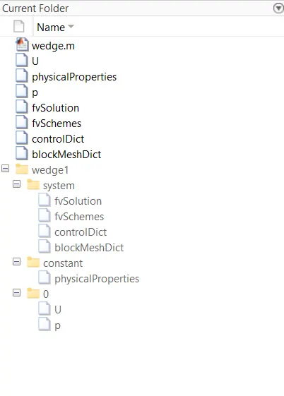
• Copy the wedge1 folder inside the OpenFoam>Run folder.
• Open terminal and access the wedge1 folder

• Run 'blockMesh' command to mesh the geometry.

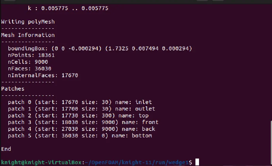
MESHING:

Front View :

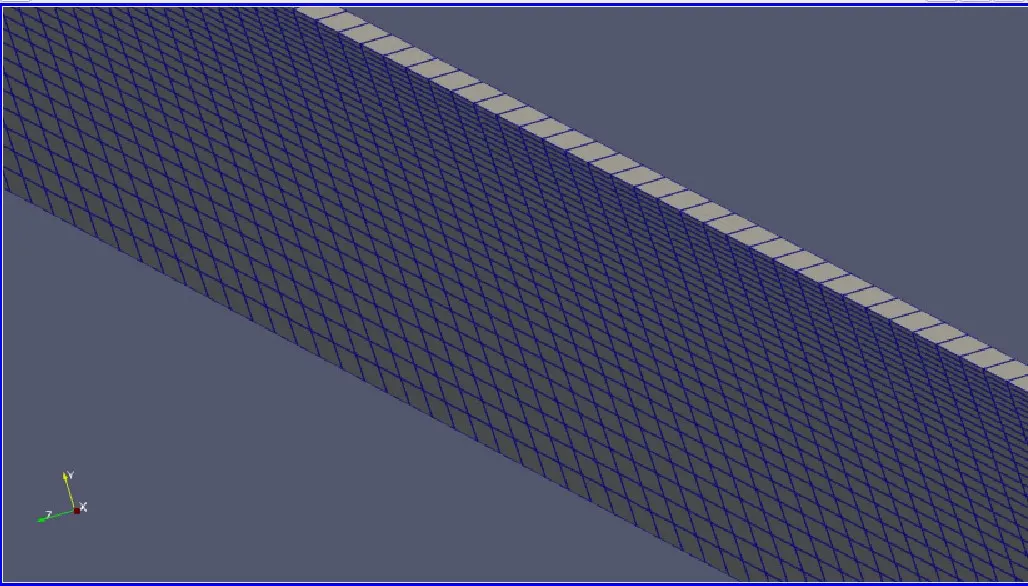
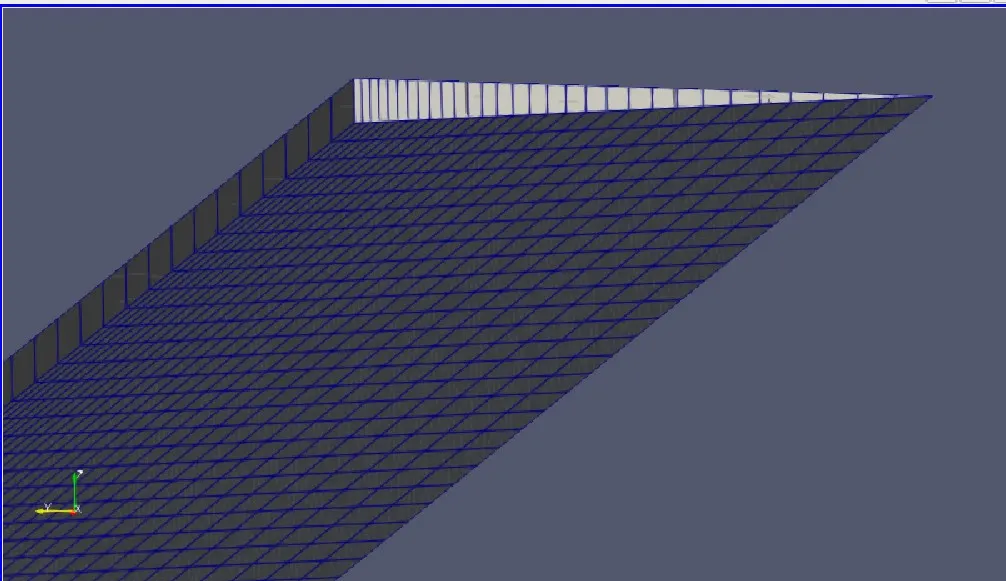
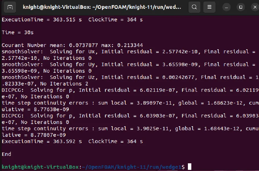
Now run the 'icoFoam" command to run the simulation:

• Open paraView using paraFoam command:

Computing all datas we get:

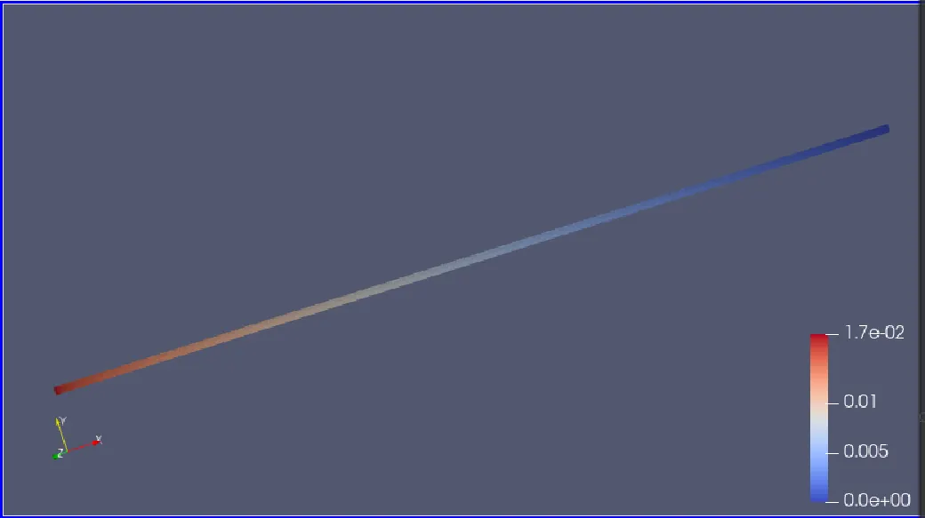
Velocity Profile:

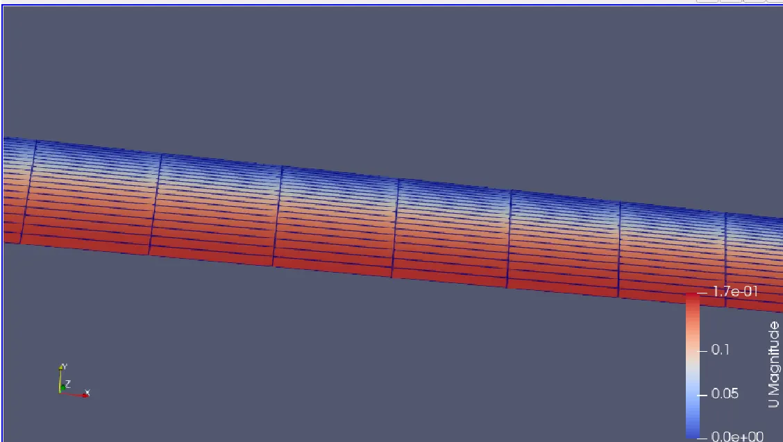
Pressure:

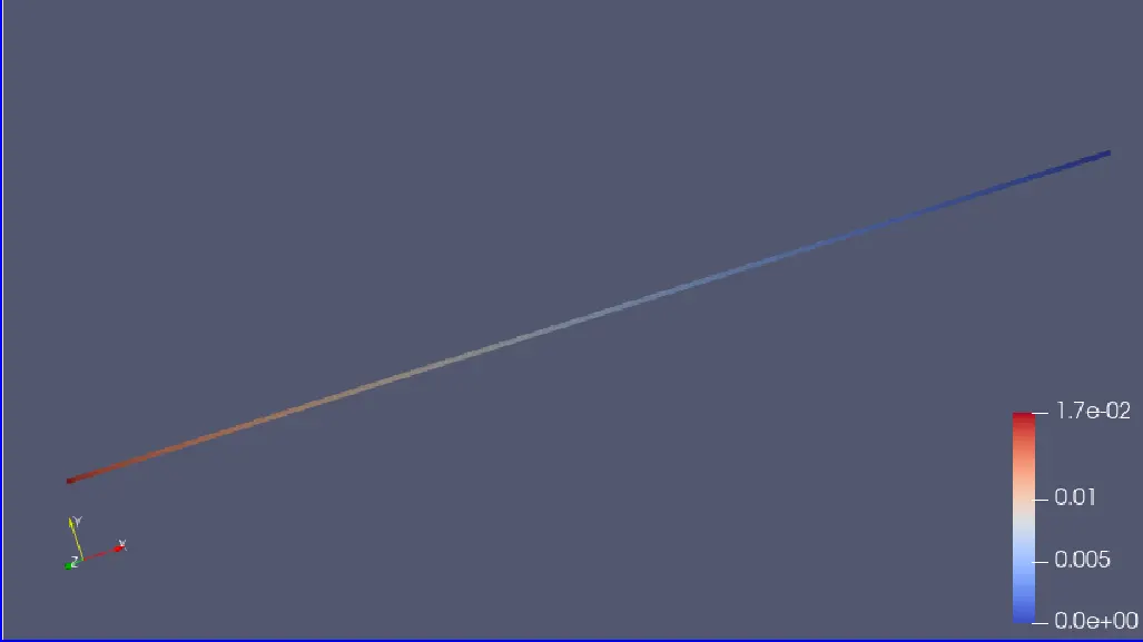
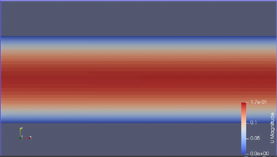
After mirroring the pipe:

Velocity profile:

---------------------------------------------------------------------------------------------------------------------------------------

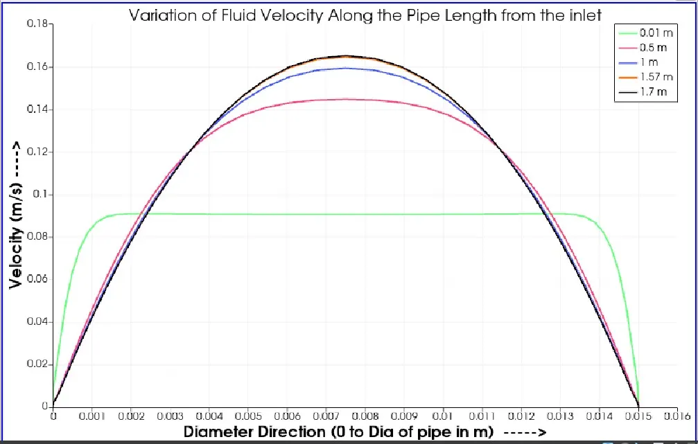
Velocity profile using ParaFoam:

ANALYTICAL: Plot for fully developed region:

---------------------------------------------------------------------------------------------------------------------------------------

Pressure:

Analytical pressure:

Using Haigen poisuelle flow equations

Avg velocity, V_avg=`(Re*mu)/(rho*d)`=0.084 m/s

Maximum velocity, Vmax=2*V_avg =0.168 m/s

Piezo metric pressure drop, `gradp=(32*mu*V_(avg)*0.1*Lhydro)/d^2``=0.8571 Pa

Kinematic pressure, Kinematic_p=`gradp`/rho=0.0011 Pa

Pressure plot using ParaFoam:

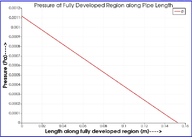
Numerical pressure at fully developed region along length: 0.001107 Pa

---------------------------------------------------------------------------------------------------------------------------------------

Shear-stress plot using ParaFoam:

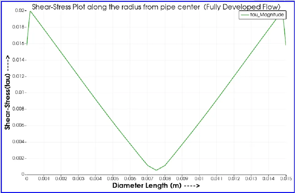
Numerical shear stress: 0.0197 N/m^2

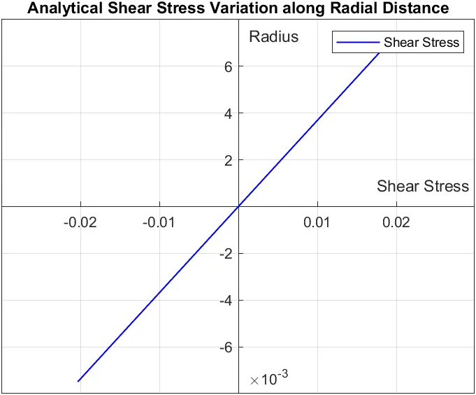
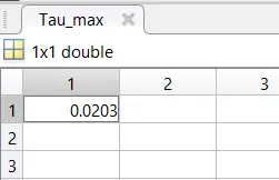
Maximum analytical shear stress:

RESULTS:

	Maximum Velocity (m/s)	Pressure Loss (Pa)	Max Shear Stress (Pa)
Numerical Results	0.165	0.001107	0.0197
Theoretical Results	0.1680	0.0011	0.0203
%Error	1.7%	0.06%	2%

As the errors are less than 5%, the numerical results are accepted.

CONCLUSION:

• Accurate CFD Analysis: Our CFD analysis provides results that closely match theoretical expectations, demonstrating the precision and reliability of our models and numerical techniques.
• Parabolic Velocity Profiles: The observed velocity profiles, particularly in fully developed flow regions, exhibit a characteristic parabolic shape. This parabolic profile signifies that the fluid flow has reached a steady state, with no further alterations in velocity distribution beyond a certain distance from the inlet.
• Entry Length Determination: In the scope of this project, we have identified that the entry length for flow in the pipe is approximately 1.57 meters. Beyond this point, the velocity distribution stabilizes into its well-defined parabolic shape, with the maximum velocity occurring at the central axis of the pipe.
• Shear Stress Impact: Shear stress plays a pivotal role in this fluid flow phenomenon. It contributes significantly to the friction experienced by the pipe walls, leading to distinct variations in velocity across the pipe's cross-section. The shear stress plot, generated during the post-processing phase, provides clear visual evidence of this distribution.
• Max Velocity at Pipe Center: As a direct result of the interplay between shear stress and wall friction, the velocity is highest at the central region of the pipe. In this region, shear stress is lowest, allowing for the maximum flow velocity. Conversely, velocity gradually decreases as one moves toward the pipe walls where shear stress reaches its maximum.