Week 8 - Simulation of a backward facing step in OpenFOAM
Courant-Friedrichs-Lewy (CFL):
It is an essential requirement when solving Partial Differential Equations (PDEs) through numerical methods. This condition emerges during the numerical analysis of explicit time integration schemes.
The Courant-Friedrichs-Lewy (CFL) number serves as a critical indicator of instability within a specific problem. Essentially, it sets the stability threshold for a reliable solution.
`C = c frac{Deltat}{Deltax}le 1`
The general CFL condition for numerical equations states that Δt should be less than or equal to Δx divided by c, where C is the Courant number. This condition is known as the Courant-Friedrichs-Lewy condition.
Grading Factor or Expansion Ratios:
The expansion ratios allow the mesh to be graded or refined in specified directions. The ratio is defined as the width of the end cell (`δ_e`) along one edge of a block to the width of the start cell (`δ_s`) along the same edge, as shown in the figure below.
In a simpler format, the expansion ratio can be understood as:
Expansion Ratio = (Size of End Cell) / (Size of Starting Cell)
AIM:
Simulate incompressible, laminar, and viscous flow through a backward-facing step. Perform transient simulations and explain setup changes. Conduct two case studies: one without grading (GF = 1) and one with GF = 0.2, focusing on wall refinement.
Objective: Find OpenFOAM solver for incompressible-laminar-viscous flow. Copy solver files, set up domain mesh, configure time parameters, initialize variables, generate and verify mesh, visualize in ParaView, and compare results for both cases and to simulate incompressible-laminar-viscous flow through a backward-facing step. Perform two case studies: one without grading (GF = 1) and one with GF = 0.2, refining cells near walls.
Mesh Specification: X-direction cells = 200, Y-direction cells = 20.
Step:
To begin the simulation process, open the terminal on your Linux operating system. You can do this by either using the keyboard shortcut "Ctrl + Alt + T" or by right-clicking on the desktop and selecting "Open Terminal." When you do this, you will see the terminal window appear on your screen.
In the terminal window, please type 'tut' and press 'Enter' to access the tutorial folder. Then, use 'ls' to display all the directories. Now, open the 'legacy' directory by typing 'cd legacy/' and utilize 'ls' to view its sub-directories. Given that the goal is to simulate incompressible-laminar-viscous flow through the backward-facing step geometry, proceed to the 'incompressible' directory by entering 'cd incompressible.'
In the provided image below, we can observe numerous solver folders. To address our specific needs for simulating laminar-viscous flow, we'll opt for 'icoFoam.'
'icoFoam' is the solver in OpenFOAM designed for transient simulations of incompressible, laminar flow involving Newtonian fluids.
(A Newtonian fluid is one in which the viscous stress induced by its flow at each point is directly proportional to the local strain rate, which is the rate of deformation change over time. Newtonian fluids represent the simplest mathematical model for fluids accounting for viscosity.)
To access the 'icoFoam' folder, we'll type 'cd icoFoam,' and to explore its contents in the terminal, we'll type 'ls.'
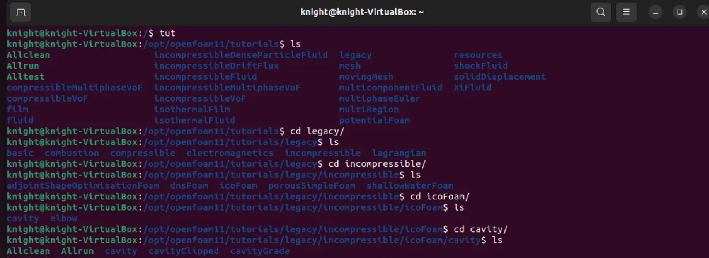
In the 'cavity' section of the 'icoFoam' solver, we have two options: 'cavity' and 'elbow.' Both are part of the icoFoam solver, but we will select the 'cavity' folder
Inside the 'cavity' folder, we will find another 'cavity' folder where we define our fluid domain and generate the block mesh. However, it's essential to note that we won't make any changes to the tutorial section. OpenFOAM does not allow modifications to its official tutorials, and attempting to do so could potentially corrupt the OpenFOAM installation. In such cases, a reinstallation may be required.
Instead, we will copy the 'cavity' folder using the 'cp -r cavity' command and paste it into the OpenFOAM run folder with 'cp -r cavity $FOAM_RUN/cavitytest.' Next, navigate to the run folder using 'cd $FOAM_RUN,' where you will find the 'cavitytest' folder.
Now that we have the 'cavity_test' folder, we can make changes to it without affecting the official OpenFOAM files. Open the 'cavitytest' folder, and inside it, we can provide specifications for our block mesh in the 'system' folder.

As shown in the picture above, there are four script files in the 'system' folder. To create the domain and specify the necessary parameters for the block mesh, open the 'blockMeshDict' file by typing 'gedit blockMeshDict.'
It's important to note that the 'blockMeshDict' file serves as a script that encompasses information related to various aspects of the geometry.
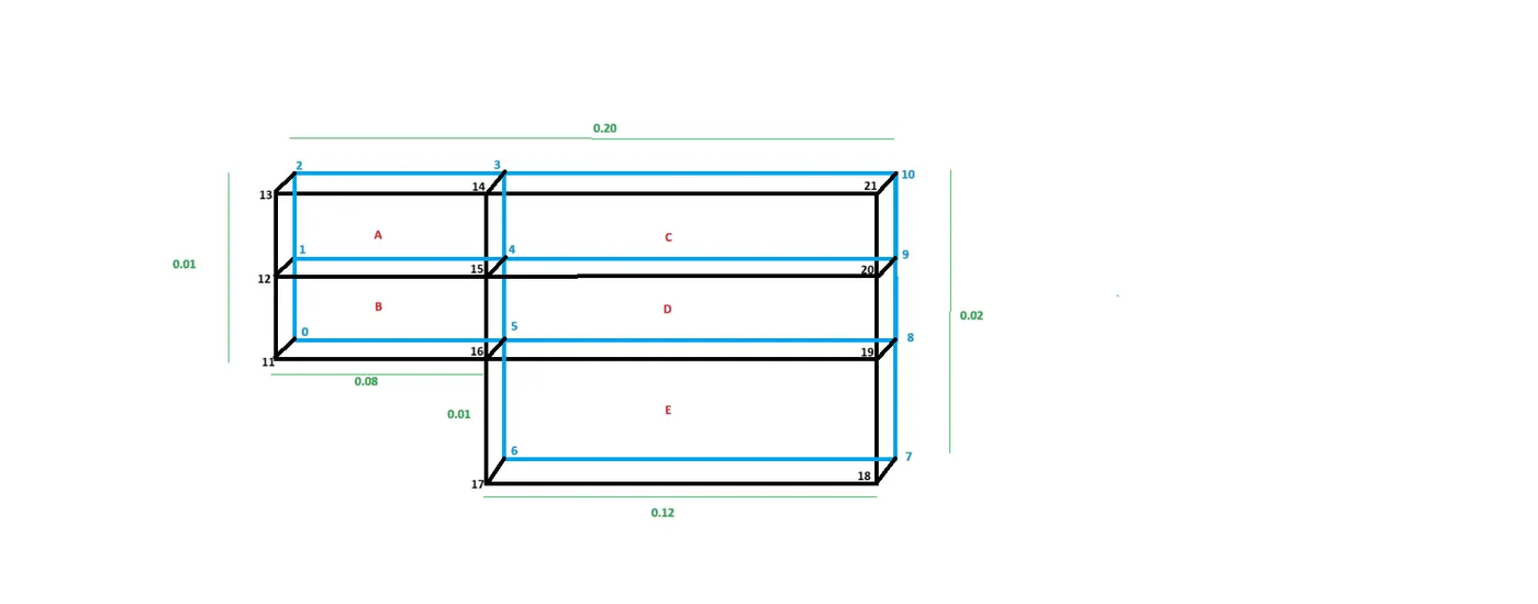
Next, we need to define the vertices for our geometry. In the code, we specify the x, y, and z coordinates for each vertex, and we always start from the origin point 0 as (0,0,0). The geometry we want to create is shown in the figure above.
To construct this geometry, we'll break it down into five blocks, as illustrated in the figure below.
Now edit the codes of blockMeshDict:
Changes done in the blockMesh script:
- It starts by setting the unit of measurement to meters, value 1 is taken as the dimensions given are in meters.
- Define the positions of 22 points (vertices) that will form the corners of our grid with refrence point vertex 0.
- The main part is where it defines blocks.The vertices are the key building blocks of the mesh. They define the corners and shape of the mesh blocks. Each block is a rectangular shape made up of vertices.The provided code defines five hexahedral blocks labeled as A, B, C, D, and E.
-
Using the above figure as reference specifying local (x,y,z) coordinates of for each block using vertex 0 as refrence, let's proceed to define the vertices for each of these blocks by referring to the sketch. :
(0.00 0.00 0.00) // Vertex 0
(0.00 0.005 0.00) // Vertex 1
(0.00 0.01 0.00) // Vertex 2
(0.08 0.01 0.00) // Vertex 3
(0.08 0.005 0.00) // Vertex 4
(0.08 0.00 0.00) // Vertex 5
(0.08 -0.01 0.00) // Vertex 6
(0.20 -0.01 0.00) // Vertex 7
(0.20 0.00 0.00) // Vertex 8
(0.20 0.005 0.00) // Vertex 9
(0.20 0.01 0.00) // Vertex 10
(0.00 0.00 0.01) // Vertex 11
(0.00 0.005 0.01) // Vertex 12
(0.00 0.01 0.01) // Vertex 13
(0.08 0.01 0.01) // Vertex 14
(0.08 0.005 0.01) // Vertex 15
(0.08 0.00 0.01) // Vertex 16
(0.08 -0.01 0.01) // Vertex 17
(0.20 -0.01 0.01) // Vertex 18
(0.20 0.00 0.01) // Vertex 19
(0.20 0.005 0.01) // Vertex 20
(0.20 0.01 0.01) // Vertex 21
- Each block is defined by vertex indices, dimensions, and grid grading factors as mentioned before.
-
In the mesh format, the first letter inside the block parenthesis is 'hex,' which defines the type of mesh as a hexahedral mesh.
Following that, inside the parenthesis, we provide the vertex numbers in a specific order that follows the right-hand thumb rule. In this rule, the thumb represents the z-axis, and the order of vertices follows the rotational order of our other fingers.
Then, we specify the number of mesh grid divisions along the x, y, and z directions in the format (nx, ny, nz).
The simple description indicates uniform expansion in the local x, y, and z directions with only 3 expansion ratios. For the first case, we won't provide any grading for our problem.
So, in this case, we have 5 blocks, so we need to define a hex mesh for these 5 blocks.
hex (1 4 3 2 12 15 14 13) (80 10 1) simpleGrading (1 1 1) // Block A
hex (0 5 4 1 11 16 15 12) (80 10 1) simpleGrading (1 1 1) // Block B
hex (4 9 10 3 15 20 21 14) (120 10 1) simpleGrading (1 1 1) // Block C
hex (5 8 9 4 16 19 20 15) (120 10 1) simpleGrading (1 1 1) // Block D
hex (6 7 8 5 17 18 19 16) (120 20 1) simpleGrading (1 1 1) // Block E
- "boundary": This section defines boundary patches and their associated boundary conditions.
The patches are named "inlet," "outlet," "frontAndBack," and "fixedWalls," each with specific faces (a list of face indices).
(a)"inlet" and "outlet" are specified as patch types with associated faces. These patches represent inlet and outlet boundaries with specified faces where the boundary conditions will be applied.
(b)"frontAndBack" is specified as an empty (type empty) patch, indicating it doesn't have specific boundary conditions. It defines the front and back faces of the blocks.
(c)"fixedWalls" is specified as a wall boundary type with associated faces, representing wall boundaries with specified faces.
type patch;:
The "patch" type is quite versatile when it comes to defining boundary conditions.This type is used to define a general boundary condition patch. It can be associated with various boundary conditions, depending on the specific case and solver used.A "patch" type is often used when you need to customize the boundary condition behavior further in the solver settings.
type empty;:
The "empty" type is used to define an empty boundary condition.This means that there is no interaction with the boundary; it's as if it doesn't exist. Typically, this type is used for patches representing far-field boundaries where no physical interaction occurs.
type wall;:
The "wall" type is used for solid boundaries where fluid interacts with the surface. It represents a no-slip condition, where the fluid velocity at the wall is equal to the velocity of the wall itself. Wall boundaries are essential for accurately modeling fluid flow around solid objects. - These type options play a pivotal role in defining how the fluid behaves at different boundary patches within a computational fluid dynamics (CFD) simulation, and they are selected based on the specific physical conditions and behavior you want to simulate.
- we have to specify the faces of our 3D block in a certain order, following the right-hand thumb rule.
inlet>type patch
(2 1 12 13) // Inlet A
(1 0 11 12) // Inlet B
outlet>type patch
(9 10 21 20) // Outlet C
(8 9 20 19) // Outlet D
(7 8 19 18) // Outlet E
frontAndBack>type empty
(13 12 15 14) //Block A front
(2 3 4 1) //Block A back
(12 11 16 15) //Block B Front
(1 4 5 0) // Block B back
(14 15 20 21) // Block C front
(3 10 9 4) // Block C back
(15 16 19 20) // Block D front
(4 9 8 5) // Block D back
(16 17 18 19) // Block E front
(5 8 7 6) // Block E back
fixedWalls> type wall
(3 2 13 14) //Top of Block A
(10 3 14 21) //Top of Block C
(0 5 16 11) //Bottom of Block B
(5 6 17 16) // front of the Block E
(6 7 18 17) //Bottom of the Block E
- The file can specify how these different areas should behave, like whether they're open or have specific conditions.
.
/*--------------------------------*- C++ -*----------------------------------*\
  =========                 |
  \\      /  F ield         | OpenFOAM: The Open Source CFD Toolbox
   \\    /   O peration     | Website:  https://openfoam.org
    \\  /    A nd           | Version:  11
     \\/     M anipulation  |
\*---------------------------------------------------------------------------*/
FoamFile
{
    format      ascii;
    class       dictionary;
    object      blockMeshDict;
}
// * * * * * * * * * * * * * * * * * * * * * * * * * * * * * * * * * * * * * //

convertToMeters 1;

vertices
(
    (0.00 0.00 0.00)  // Vertex 0
    (0.00 0.005 0.00) // Vertex 1
    (0.00 0.01 0.00)  // Vertex 2
    (0.08 0.01 0.00)  // Vertex 3
    (0.08 0.005 0.00) // Vertex 4
    (0.08 0.00 0.00)  // Vertex 5
    (0.08 -0.01 0.00) // Vertex 6
    (0.20 -0.01 0.00) // Vertex 7
    (0.20 0.00 0.00)  // Vertex 8
    (0.20 0.005 0.00) // Vertex 9
    (0.20 0.01 0.00)  // Vertex 10
    (0.00 0.00 0.01)  // Vertex 11
    (0.00 0.005 0.01) // Vertex 12
    (0.00 0.01 0.01)  // Vertex 13
    (0.08 0.01 0.01)  // Vertex 14
    (0.08 0.005 0.01) // Vertex 15
    (0.08 0.00 0.01)  // Vertex 16
    (0.08 -0.01 0.01) // Vertex 17
    (0.20 -0.01 0.01) // Vertex 18
    (0.20 0.00 0.01)  // Vertex 19
    (0.20 0.005 0.01) // Vertex 20
    (0.20 0.01 0.01)  // Vertex 21
);

edges
(
);

blocks
(
    hex (1 4 3 2 12 15 14 13) (80 10 1) simpleGrading (1 1 1) // Block A
    hex (0 5 4 1 11 16 15 12) (80 10 1) simpleGrading (1 1 1) // Block B
    hex (4 9 10 3 15 20 21 14) (120 10 1) simpleGrading (1 1 1) // Block C
    hex (5 8 9 4 16 19 20 15) (120 10 1) simpleGrading (1 1 1) // Block D
    hex (6 7 8 5 17 18 19 16) (120 20 1) simpleGrading (1 1 1) // Block E
);

boundary
(
    inlet
    {
        type patch;
        faces
        (
            (2 1 12 13) // Inlet A
            (1 0 11 12) // Inlet B
        );
    }

    outlet
    {
        type patch;
        faces
        (
            (9 10 21 20) // Outlet C
            (8 9 20 19) // Outlet D
            (7 8 19 18) // Outlet E
        );
    }
 frontAndBack
 {
  type empty;
  faces
  (
   (13 12 15 14) //Block A front
   (2 3 4 1) //Block A back
   (12 11 16 15) //Block B Front
   (1 4 5 0) // Block B back
   (14 15 20 21) // Block C front
   (3 10 9 4) // Block C back
   (15 16 19 20) // Block D front
   (4 9 8 5) // Block D back
   (16 17 18 19) // Block E front
     (5 8 7 6) // Block E back
    );
    }

 fixedWalls
 {
    type wall;
    faces
    (
     (3 2 13 14) //Top  of Block A
     (10 3 14 21) //Top of Block C
     (0 5 16 11) //Bottom of Block B
     (5 6 17 16) // front of the Block E
     (6 7 18 17) //Bottom of the Block E

     );
     }
     );
 mergePatchPairs
(
);

// ****************************************************** //
Next, we will edit the 'controlDict' file to set time limits (start time and end time) and specify the time step size (deltaT). When selecting the deltaT value, ensure that the Courant-Friedrichs-Lewy (CFL) number is less than 1. If the CFL value exceeds 1, it may lead to the solution being forcibly stopped or divergence during the convergence process. Therefore, make the following changes in the 'controlDict' file.
- File: controlDict
It Specifies control settings for the simulation. - Application: icoFoam
The chosen application for this simulation is icoFoam, which is a solver specifically designed for incompressible, laminar flow simulations.
Changes to be made in the controlDict File:
Simulation Time Control - startTime= 0
The simulation will commence from time zero (0) as specified in startTime. - endTime= 5
The simulation is configured to run until reaching an end time of 5 seconds, controlled by endTime. - deltaT= 2e-4 (0.0002)
The time step size for the simulation is set to 2e-4 (0.0002) units, defined by deltaT. - Write Control= timeStep
Output data will be written at specified time steps, determined by timeStep. - Write Interval=500
Output data will be written at intervals of 500 time steps. - Floating-point data in the output will be displayed with a precision of 6 decimal places.
- Time Format and Precision is given value upto 6 decimal places
- Run-Time Modifiability: Enabled (true)
The simulation is set to be modifiable during runtime. This means that boundary conditions, turbulence models, and other settings can be adjusted while the simulation is running.
These control settings collectively define the behavior of the CFD simulation, ensuring it starts and stops at the desired times, maintains specified time step sizes, and produces output data in the desired format and precision. Additionally, the ability to modify simulation parameters during runtime enhances flexibility in experimentation and analysis.

This information should be added to the script file as follows:
/*--------------------------------*- C++ -*----------------------------------*\
  =========                 |
  \\      /  F ield         | OpenFOAM: The Open Source CFD Toolbox
   \\    /   O peration     | Website:  https://openfoam.org
    \\  /    A nd           | Version:  11
     \\/     M anipulation  |
\*---------------------------------------------------------------------------*/
FoamFile
{
    format      ascii;
    class       dictionary;
    location    "system";
    object      controlDict;
}
// * * * * * * * * * * * * * * * * * * * * * * * * * * * * * * * * * * * * * //

application     icoFoam;

startFrom       startTime;

startTime       0;

stopAt          endTime;

endTime         2;

deltaT          2e-5;

writeControl    timeStep;

writeInterval   20;

purgeWrite      0;

writeFormat     ascii;

writePrecision  6;

writeCompression off;

timeFormat      general;

timePrecision   6;

runTimeModifiable true;


// ************************************************************************* //
Next, it is needed to establish the initial values for pressure and velocity. To achieve this, let's navigate back to the 'cavitytest' directory by using the 'cd ..' command. Inside the 'cavitytest' directory, locate the folder named '0,' which represents the initial values for pressure and velocity.
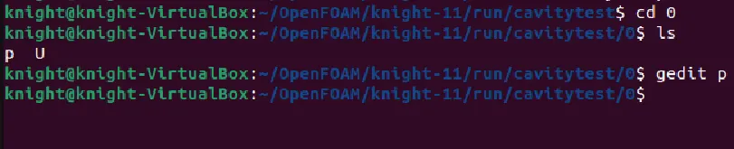
Changes made in the p file:
- object p;: Indicates that the field being defined is the pressure field denoted as "p."
- dimensions [0 2 -2 0 0 0 0];: This line defines the dimensions of the pressure field. The numbers in the brackets represent dimensions in the order [M L T Θ N J I], where M stands for mass, L for length, T for time, Θ for temperature, N for quantity, J for current, and I for luminous intensity. In this case, it represents a dimensionless quantity with dimensions [0 2 -2 0 0 0 0], indicating pressure (M L^-1 T^-2).
- internalField uniform 0;: Specifies the initial value of the pressure field within the computational domain. In this case, it's initialized with a uniform value of 0.
- boundaryField: This section defines the boundary conditions for different parts of the computational domain.
- inlet: This boundary condition is applied to the inlet boundary.
- type zeroGradient;: Specifies that the pressure gradient at the inlet is zero, which is often used for pressure boundaries that are open to the environment.
- outlet: This boundary condition is applied to the outlet boundary.
- type fixedValue;: Indicates that the pressure is held fixed at the specified value.
- value uniform 0;: Sets the pressure at the outlet to a uniform value of 0.
- frontAndBack: This boundary type is set to "empty," indicating that there are no specific pressure conditions specified for the front and back boundaries.
- fixedWalls: This boundary type is set to "zeroGradient," meaning that the pressure gradient on the walls is zero, which is a common condition for solid walls.
/*--------------------------------*- C++ -*----------------------------------*\
  =========                 |
  \\      /  F ield         | OpenFOAM: The Open Source CFD Toolbox
   \\    /   O peration     | Website:  https://openfoam.org
    \\  /    A nd           | Version:  11
     \\/     M anipulation  |
\*---------------------------------------------------------------------------*/
FoamFile
{
    format      ascii;
    class       volScalarField;
    object      p;
}
// * * * * * * * * * * * * * * * * * * * * * * * * * * * * * * * * * * * * * //

dimensions      [0 2 -2 0 0 0 0];

internalField   uniform 0;

boundaryField
{
inlet
    {
        type  zeroGradient;
    }


    outlet
    {
        type   fixedValue;
        value  uniform 0;
    }
 frontAndBack
 {
  type  empty;

    }

 fixedWalls
 {
    type  zeroGradient;

     }
     }

// ************************************************************************* //
Now access velocity file U and set velocity to 1 m/s.

Change made in U file :
- object U;: Indicates that the field being defined is the velocity field denoted as "U."
- dimensions [0 1 -1 0 0 0 0];: This line defines the dimensions of the velocity field. The numbers in the brackets represent dimensions in the order [M L T Θ N J I], where M stands for mass, L for length, T for time, Θ for temperature, N for quantity, J for current, and I for luminous intensity. In this case, it represents a field with dimensions [0 1 -1 0 0 0 0], which corresponds to velocity (L T^-1).
- internalField uniform (0 0 0);: Specifies the initial value of the velocity field within the computational domain. It's initialized with a uniform velocity vector of (0 0 0), indicating zero velocity in all three Cartesian directions (x, y, z).
- boundaryField: This section defines the boundary conditions for different parts of the computational domain.
- inlet: This boundary condition is applied to the inlet boundary.
- type fixedValue;: Specifies that the velocity at the inlet is held fixed at the specified value.
- value uniform (1 0 0);: Sets the velocity at the inlet to a uniform value of (1 0 0), indicating a velocity of 1 m/s in the x-direction and zero velocity in the y and z directions.
- outlet: This boundary condition is applied to the outlet boundary.
- type zeroGradient;: Indicates that the velocity gradient at the outlet is zero, which is often used for pressure boundaries that are open to the environment.
- frontAndBack: This boundary type is set to "empty," indicating that there are no specific velocity conditions specified for the front and back boundaries.
- fixedWalls: This boundary type is set to "noSlip," meaning that the velocity at the walls is zero, indicating a no-slip condition.
/*--------------------------------*- C++ -*----------------------------------*\
  =========                 |
  \\      /  F ield         | OpenFOAM: The Open Source CFD Toolbox
   \\    /   O peration     | Website:  https://openfoam.org
    \\  /    A nd           | Version:  11
     \\/     M anipulation  |
\*---------------------------------------------------------------------------*/
FoamFile
{
    format      ascii;
    class       volVectorField;
    object      U;
}
// * * * * * * * * * * * * * * * * * * * * * * * * * * * * * * * * * * * * * //

dimensions      [0 1 -1 0 0 0 0];

internalField   uniform (0 0 0);

boundaryField
{
     inlet
    {
      type            fixedValue;
        value           uniform (1 0 0);
    }


    outlet
    {
        type            zeroGradient;

    }
 frontAndBack
 {
  type  empty;
    }

  fixedWalls
    {
        type            noSlip;

    }

}

// ************************************************************************* //
At this point, our problem statement is configured, and we can proceed to generate the mesh using the 'blockMesh' command. After mesh generation, it's advisable to use the 'checkMesh' command to ensure that there are no errors or issues in our mesh.
Using 'blockMesh':

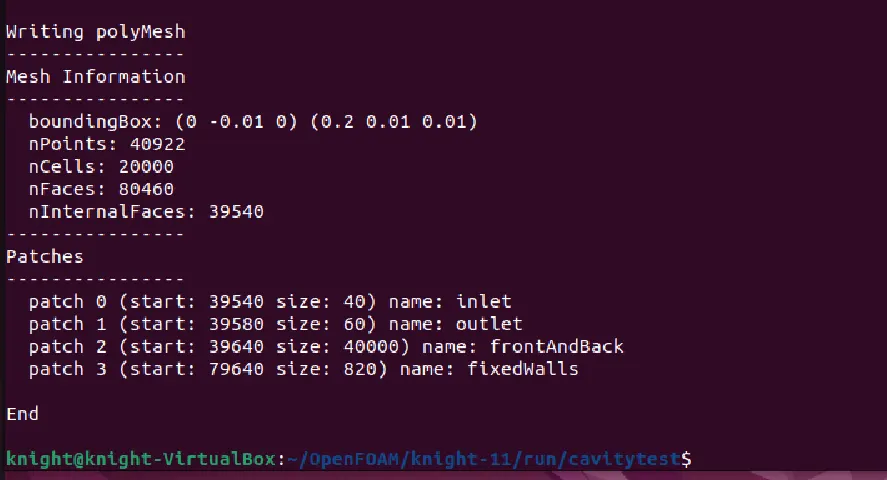
Using 'checkMesh':

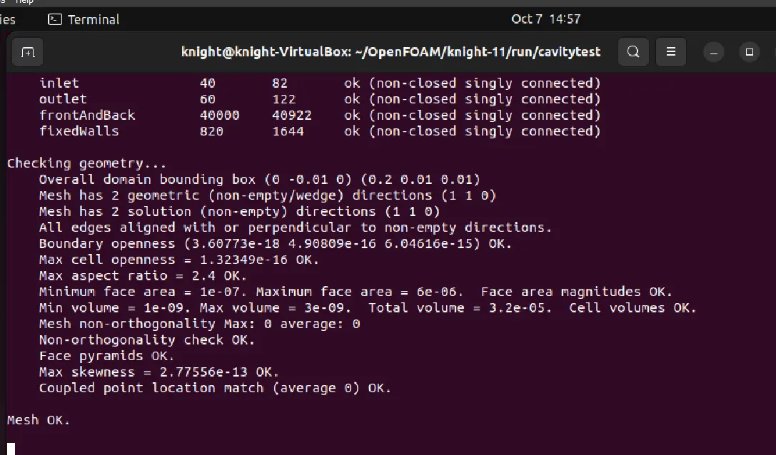
As the checkMesh command doesn't detect any error. Next step is to start simulation using 'icoFoam' command.
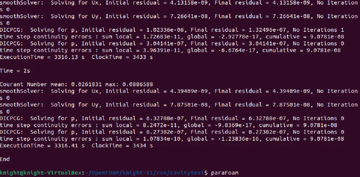
Now to view the results in ParaView use 'paraFoam' command to command.
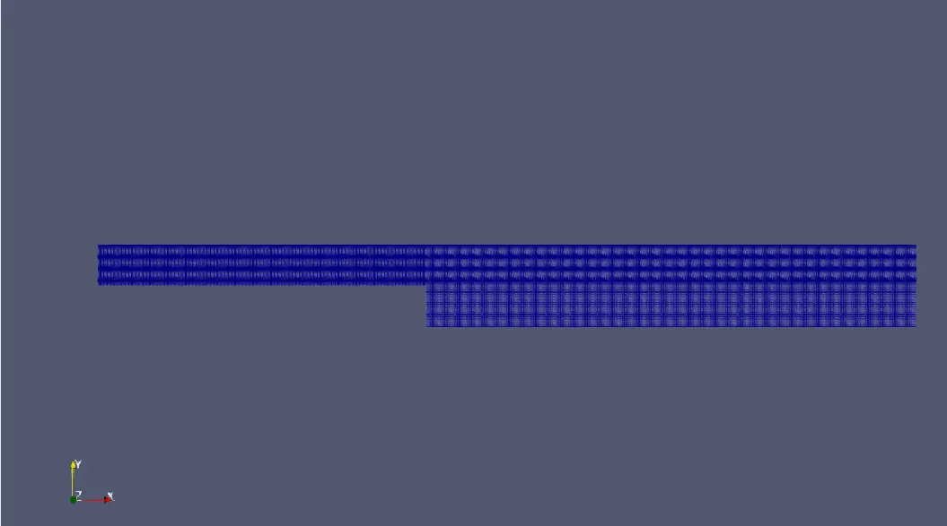
Mesh grid:-
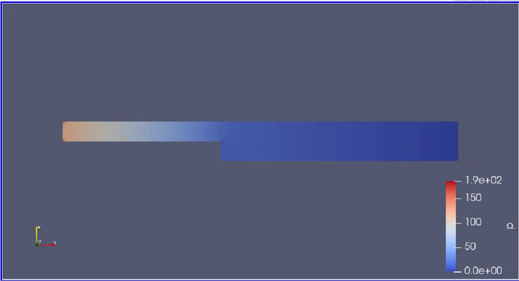
Pressure Distribution along the domain area:-
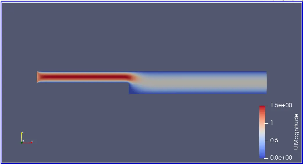
Velocity Distribution along the domain area:-
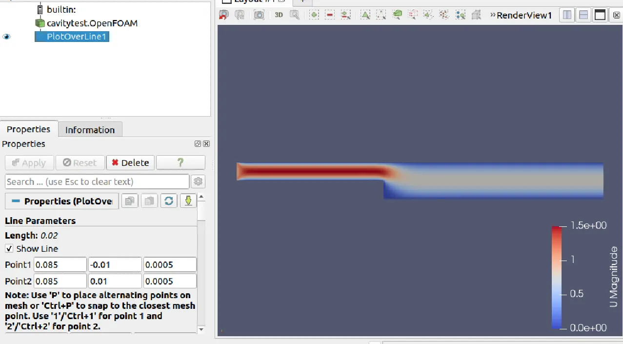
To Calculate velocity at distance 0.085 from inlet modify following parameters.
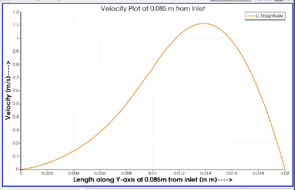
Velocity Plot:-
---------------------------------------------------------------------------------------------------------------------------------------
With Grading Factor 0.2 (cell near fixed walls)
Now, lets solve same problem for grading factor 0.2.
To get a mesh with 0.2 grading on the same geometry we need to change the grading factor values in the blockMeshDict file as given below
blocks
(
hex (1 4 3 2 12 15 14 13) (80 10 1) simpleGrading (1 0.2 1) // Block A
hex (0 5 4 1 11 16 15 12) (80 10 1) simpleGrading (1 5 1) // Block B
hex (4 9 10 3 15 20 21 14) (120 10 1) simpleGrading (5 0.2 1) // Block C
hex (5 8 9 4 16 19 20 15) (120 10 1) simpleGrading (5 5 1) // Block D
hex (6 7 8 5 17 18 19 16) (120 20 1) simpleGrading (5 5 1) // Block E
);
Here the global X-Y axis are taken into consideration for deciding the first layer and end layer in the geometry. The grading is done in such a way so that the cell alignment in the whole geometry is not misaligned.
Making change in the previous blockMeshDict file:
/*--------------------------------*- C++ -*----------------------------------*\
  =========                 |
  \\      /  F ield         | OpenFOAM: The Open Source CFD Toolbox
   \\    /   O peration     | Website:  https://openfoam.org
    \\  /    A nd           | Version:  11
     \\/     M anipulation  |
\*---------------------------------------------------------------------------*/
FoamFile
{
    format      ascii;
    class       dictionary;
    object      blockMeshDict;
}
// * * * * * * * * * * * * * * * * * * * * * * * * * * * * * * * * * * * * * //

convertToMeters 1;

vertices
(
    (0.00 0.00 0.00)  // Vertex 0
    (0.00 0.005 0.00) // Vertex 1
    (0.00 0.01 0.00)  // Vertex 2
    (0.08 0.01 0.00)  // Vertex 3
    (0.08 0.005 0.00) // Vertex 4
    (0.08 0.00 0.00)  // Vertex 5
    (0.08 -0.01 0.00) // Vertex 6
    (0.20 -0.01 0.00) // Vertex 7
    (0.20 0.00 0.00)  // Vertex 8
    (0.20 0.005 0.00) // Vertex 9
    (0.20 0.01 0.00)  // Vertex 10
    (0.00 0.00 0.01)  // Vertex 11
    (0.00 0.005 0.01) // Vertex 12
    (0.00 0.01 0.01)  // Vertex 13
    (0.08 0.01 0.01)  // Vertex 14
    (0.08 0.005 0.01) // Vertex 15
    (0.08 0.00 0.01)  // Vertex 16
    (0.08 -0.01 0.01) // Vertex 17
    (0.20 -0.01 0.01) // Vertex 18
    (0.20 0.00 0.01)  // Vertex 19
    (0.20 0.005 0.01) // Vertex 20
    (0.20 0.01 0.01)  // Vertex 21
);

edges
(
);

blocks
(
    hex (1 4 3 2 12 15 14 13) (80 10 1) simpleGrading (1 0.2 1) // Block A
    hex (0 5 4 1 11 16 15 12) (80 10 1) simpleGrading (1 5 1) // Block B
    hex (4 9 10 3 15 20 21 14) (120 10 1) simpleGrading (5 0.2 1) // Block C
    hex (5 8 9 4 16 19 20 15) (120 10 1) simpleGrading (5 5 1) // Block D
    hex (6 7 8 5 17 18 19 16) (120 20 1) simpleGrading (5 5 1) // Block E
);

boundary
(
    inlet
    {
        type patch;
        faces
        (
            (2 1 12 13) // Inlet A
            (1 0 11 12) // Inlet B
        );
    }

    outlet
    {
        type patch;
        faces
        (
            (9 10 21 20) // Outlet C
            (8 9 20 19) // Outlet D
            (7 8 19 18) // Outlet E
        );
    }
 frontAndBack
 {
  type empty;
  faces
  (
   (13 12 15 14) //Block A front
   (2 3 4 1) //Block A back
   (12 11 16 15) //Block B Front
   (1 4 5 0) // Block B back
   (14 15 20 21) // Block C front
   (3 10 9 4) // Block C back
   (15 16 19 20) // Block D front
   (4 9 8 5) // Block D back
   (16 17 18 19) // Block E front
     (5 8 7 6) // Block E back
    );
    }

 fixedWalls
 {
    type wall;
    faces
    (
     (3 2 13 14) //Top  of Block A
     (10 3 14 21) //Top of Block C
     (0 5 16 11) //Bottom of Block B
     (5 6 17 16) // front of the Block E
     (6 7 18 17) //Bottom of the Block E

     );
     }
     );
 mergePatchPairs
(
);

// ****************************************************** //
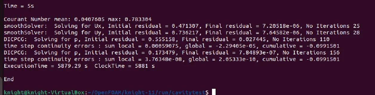
To run the simulation for 5 sec, we need to make some changes in the contolDict file as the courant number becomes high at previous setting and to reduce memory consumption and simulation time changes are made in the time-step deltaT and writeInterval values respectively.
/*--------------------------------*- C++ -*----------------------------------*\
  =========                 |
  \\      /  F ield         | OpenFOAM: The Open Source CFD Toolbox
   \\    /   O peration     | Website:  https://openfoam.org
    \\  /    A nd           | Version:  11
     \\/     M anipulation  |
\*---------------------------------------------------------------------------*/
FoamFile
{
    format      ascii;
    class       dictionary;
    location    "system";
    object      controlDict;
}
// * * * * * * * * * * * * * * * * * * * * * * * * * * * * * * * * * * * * * //

application     icoFoam;

startFrom       startTime;

startTime       0;

stopAt          endTime;

endTime         5;

deltaT          0.5e-5;

writeControl    timeStep;

writeInterval   5000;

purgeWrite      0;

writeFormat     ascii;

writePrecision  6;

writeCompression off;

timeFormat      general;

timePrecision   6;

runTimeModifiable true;


// ************************************************************************* //
Remaining p and U files as not require to chnage.
Now run the simulation using 'icoFoam' command.
Now to view the results in ParaView use 'paraFoam' command to command.
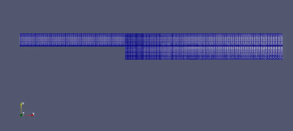
Mesh grid for 0.2 grading:-
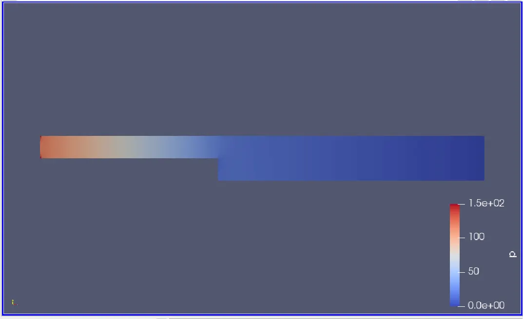
Pressure Distribution along the domain area for grading factor 0.2:-
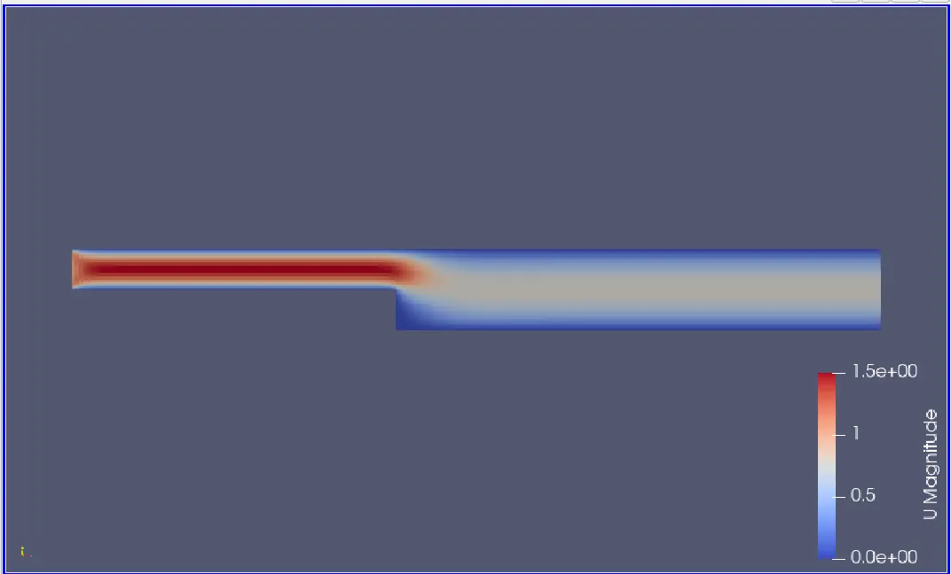
Velocity Distribution along the domain area for grading factor 0.2 at 0.085 m from inlet:-
Velocity plot for grading factor 0.2 at 0.085 m from inlet:-
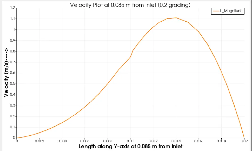
- Analyzed velocity plots for two scenarios: one without a grading factor and another with a 0.2 grading factor.
- Initial observation: Velocity plot without grading factor appeared smoother and more accurate than the other two plots. However, this initial conclusion is incorrect.
- Detailed examination reveals a critical factor: the mesh configuration.
- Mesh near the step wall along the X-axis is fine, but it becomes coarse along the Y-axis.
- Challenges in achieving a smooth velocity plot at specific points, like 0.085 along the Y-axis
CONCLUSION:
- Understanding meshing techniques highlights the importance of using finer mesh in CFD simulations.
- Fluid behavior changes significantly near walls and obstacles in CFD analysis.
- Consistently applying mesh grading near these areas is crucial for accurate representations.
Mesh Grading Strategy - Precise and dependable results require a clear understanding of effective mesh grading.
- Avoid the temptation to use an excessive number of fine mesh elements, which can increase computation time and RAM usage.
- Strategically apply mesh grading for finer mesh near walls and obstacles, and coarser mesh in simpler flow regions.
Importance of Mesh Grading - Visual representation demonstrates the significance of finer mesh resolution.
- Increasing the grading factor near a step visibly improves image resolution.
- This enhancement parallels the improved accuracy in CFD simulations with more mesh elements.