Week 3 - External flow simulation over an Ahmed body.
AIM:
To perform external flow simulation over an Ahmed body.
OBJECTIVE:
- Outline Ahmed's physique and its significance.
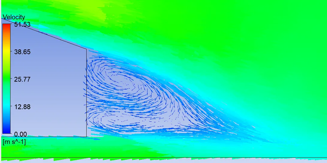
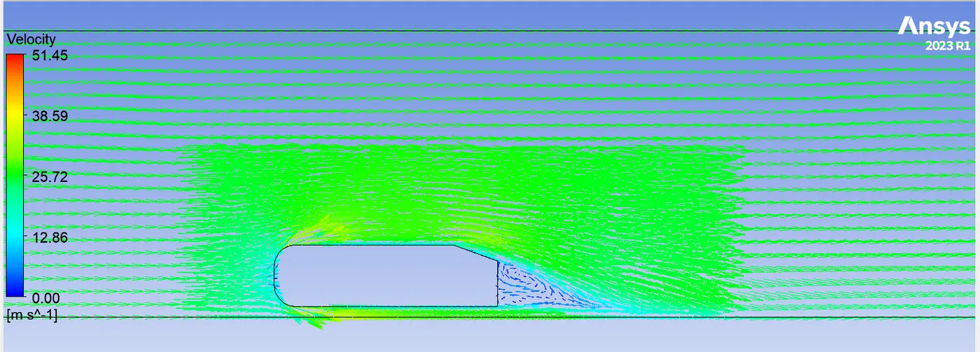
- Elaborate on the cause of negative pressure in the wake region, accompanied by a clear vector plot delineating the wake region.
- Discuss the importance of the separation point.
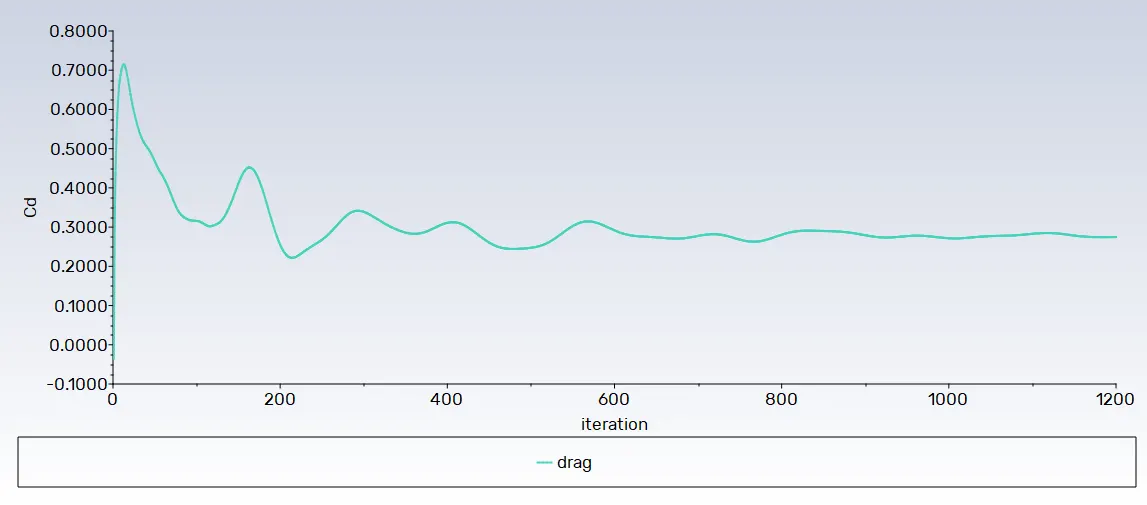
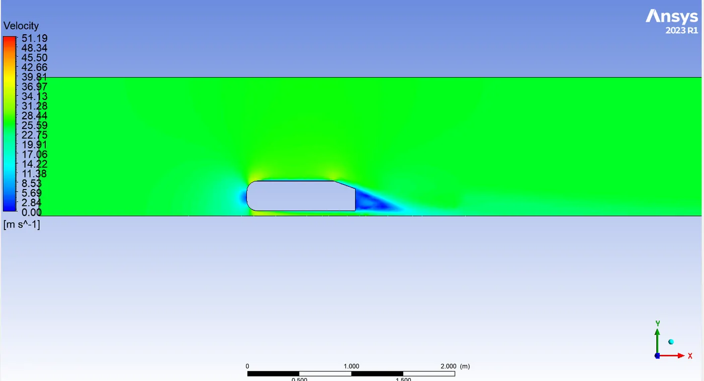
- Present velocity and pressure contours, along with the drag coefficient plot for an enhanced scenario.
- Conduct the grid independency test, furnishing drag and lift values for each case.
INTRODUCTION:
External flow in fluid mechanics refers to the unimpeded development of boundary layers around a body without constraints imposed by adjacent surfaces. Unlike internal flow, where entrance and internal flows exhibit significant viscous effects, external flows allow for the freely developing "boundary layers" in the entrance region or thin shear layers along the solid surface. These external flows can be broadly classified as those occurring over immersed bodies, such as the airflow over aircraft and ground vehicles, water flow around a submersible vessel, or the flight of footballs, golf balls, and baseballs.
A key focus in the study of external flows lies in understanding the fluid forces acting on the body, as these forces define the dynamics of objects navigating through the surrounding fluid. Despite challenges in analytical solutions, especially for higher Reynolds numbers, external flow analysis becomes particularly complex as separation regions and wakes develop even in modest laminar regimes (Re~10).
External flow scenarios encompass situations where the flow either moves over a stationary body, as in a wind tunnel experiment, or a body moves through a quiescent fluid, as observed in a flying airplane. In fluid dynamics, it is common to describe external flow in a reference frame fixed to the body, using constant upstream conditions (velocity, pressure, density) as inputs unaffected by the body's presence.
Practical external flows are often turbulent, influencing the dynamics of objects as they traverse the fluid. The impact of pressure and viscous forces becomes crucial in understanding the fluid forces acting on the object. In essence, the primary objectives in external flow analysis revolve around predicting these fluid forces and gaining insights into the underlying flow physics governing them. The challenges presented by external flow make it a persistent and intriguing problem in modern fluid dynamics.
Ahmed's body and its importance:
The Ahmed Body, a simplified car body extensively used in automotive research, plays a crucial role in understanding the intricate dynamics of external flows, particularly in the context of drag. This body serves as a model to investigate the flow patterns and their impact on drag, offering insights into the external aerodynamics of cars. The aerodynamic characteristics of a vehicle, such as stability, comfort, and fuel consumption at high speeds, are profoundly influenced by the flow around it. The Ahmed Body, designed with a round front part, a movable z slant plane in the rear for studying detachment phenomena at various angles, and a connecting rectangular box, serves as a valuable tool for comprehending the wake flow around the body.
In addition to the general insights into external flows, the Ahmed Body aids in the exploration of high turbulent and three-dimensional flow separations inherent in the aerodynamics of automobiles. The complexity of these dynamic flows necessitates a deeper understanding of their physical features. By dissecting the flow processes involved in drag production using the Ahmed Body, researchers can glean valuable information for designing cars that minimize drag. This reduction in drag not only enhances fuel efficiency but also contributes to overall vehicle performance. Consequently, the Ahmed Body stands as a critical component in the pursuit of optimizing automotive design and aerodynamic efficiency, highlighting its importance in the broader field of fluid dynamics and automotive engineering.
Significance of Ahmed Body:
The Ahmed Body stands as a pivotal tool in comprehending the fundamental physics underlying lift and drag forces, along with associated coefficients, at characteristic velocities, pressure differences, and Reynolds numbers. Engineers leverage this simplified vehicle volume to delve into the intricacies of vortices, turbulence, and flow phenomena. Utilizing the ANSYS general-purpose FEA and CFD simulation software, numerical predictions are generated, offering insights into system behavior.
Validation of these numerical predictions is crucial, and the Ahmed Body plays a central role in this process. Professionals in vehicle aerodynamics turn to the Ahmed Body to validate their numerical models, benefiting from available experimental data obtained through wind tunnel testing. Once the numerical model is validated, it becomes a valuable tool for designing new car models.
The simplicity of the Ahmed Body's shape facilitates accurate flow simulations while retaining practical features relevant to automobile bodies. This model serves as a guide for calculating turbulent flow fields around car-like geometries, employing interfaces such as Turbulent Flow, k-epsilon, and k-omega. Whether recreated experimentally or computationally, this approach allows for the exploration of desired geometries, contributing to the development of new models for market release or research purposes.
Originally described by S. R. Ahmed in 1984, the Ahmed Body exhibits three main features in its wake:
- the A recirculation region formed at the top of the vertical back surface,
- the B recirculation region resulting from separation at the base, and
- the c-pillar vortices emerging as vorticity in the side boundary layers rolls over slant edges.
The wake's characteristics are highly dependent on the slant angle, with the flow remaining attached for slant angles below 12°, becoming three-dimensional between 12° and 30°, and experiencing a sudden decrease in drag past 30° as the flow fully separates off the slant, weakening the c-pillar vortices. This detailed understanding of the wake's behavior contributes significantly to optimizing vehicle aerodynamics and performance.
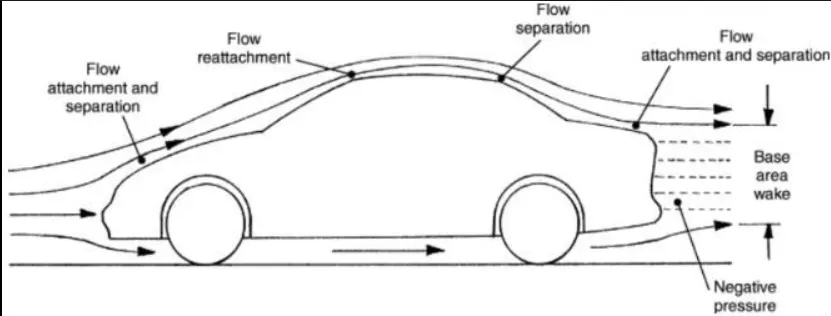
Negative Pressure in the Wake Region:
As the air flows over a moving vehicle, separation occurs at the rear end, creating a substantial turbulent area of low pressure referred to as the wake. This wake phenomenon is a crucial factor contributing to pressure drag, exerting a notable influence on the overall performance of the vehicle.
During the vehicle's motion at a specific velocity, the fluid imparts viscous forces to the vehicle within the viscous sublayer of the boundary. However, as the fluid reaches the rear end of the vehicle, detachment from the body's surface occurs, resulting in the establishment of negative pressure within the wake region. This negative pressure in the wake plays a pivotal role in the aerodynamics of the vehicle and contributes significantly to the drag experienced.
The intricate movement of the fluid around the vehicle is intricately tied to the car's geometry and the Reynolds number. Understanding and managing the negative pressure in the wake region is essential for optimizing vehicle design and minimizing the adverse effects of pressure drag on performance.
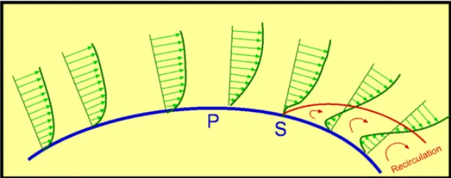
Significance of Point of Separation:
The fluid separation point is identified as the juncture where the velocity gradient (dv/dy) and the pressure gradient (dp/dx) both reach zero for a specific point. In simpler terms, it signifies the location where the velocity gradient becomes zero, and simultaneously, the pressure gradient along the x-direction becomes zero, marking the onset of separation or the formation of a negative pressure gradient beyond that point.
A more nuanced comprehension of the separation point goes beyond a single contour and involves a supportive analysis using plots of dp/dx, velocity variations with respect to the Y direction, and other relevant plots. These graphical representations provide insights into the nature of physical properties, such as regions where dp/dx=0 and dv/dy=0, within the fluid-body interaction. The complexity of fluid separation necessitates a multi-faceted approach to study and understand its occurrence, emphasizing the interplay between velocity and pressure gradients for a comprehensive analysis of separation phenomena.The point of separation holds paramount significance in understanding and optimizing the aerodynamics of a vehicle. This critical juncture arises when there is a discontinuity in the surface or a region characterized by a negative pressure gradient, often occurring at sharp ends or the rear portion of the car.
When the flow remains attached to the vehicle's body, the viscous forces increase, leading to elevated pressure and a subsequent decrease in velocity as the flow approaches the rear end. However, upon encountering a sharp turn, the velocity decreases abruptly, creating a negative pressure region in the wake area after the point of separation. This marks the initiation of a recirculation region beyond the separation point.
The efficiency of the mixing process is contingent on the rate of change of pressure; a rapid change inhibits effective mixing, leading to the cessation of the boundary layer flow. The visual representation illustrates that at the point of turning, the flow separates from the boundary layer, giving rise to a recirculation region. Beyond this region, the flow reattaches itself to the boundary layer. To mitigate fluid separation from the boundary layer and optimize aerodynamic performance, it is advisable to employ a smooth edge. A streamlined design with smooth edges reduces the impact of drag on the vehicle, emphasizing the role of the separation point in shaping vehicle efficiency and aerodynamic behavior.
How to determine `y^+`Values:
The (pronounced as "y plus") value is a dimensionless quantity used in computational fluid dynamics (CFD) simulations, particularly in the context of wall-bounded flows. It represents the dimensionless distance of the nearest grid node to the wall from the wall itself. The value is essential for determining the appropriate mesh resolution near the wall.
Desired `y^+`Values:
- Low `y^+`(e.g., `y^+`<5)
(e.g., Description: Represents a "fully-resolved" or "wall-resolved" simulation.
Why: Suitable for Direct Numerical Simulation (DNS) or Large Eddy Simulation (LES) where the smallest turbulent structures are explicitly resolved. - Moderate `y^+`(e.g., 30<`y^+`<300):
Description: Represents a "wall-modeled" or "wall-modeled LES" simulation.
Why: Suitable for Reynolds-Averaged Navier-Stokes (RANS) simulations with wall functions. Resolves larger turbulent structures and models the effects of smaller ones. - High `y^+` (e.g., `y^+`>300):
Description: Represents a "fully-modeled" or "fully-turbulent" simulation.
Why: Suitable for RANS simulations with no wall functions. All turbulent structures are modeled, and no resolution near the wall is explicitly performed.
Why Desired y +Values Matter:
- Accuracy: Achieving the desired y+ values ensures accurate representation of the near-wall flow physics.
- Boundary Layer Resolution: Proper `y^+` values help in resolving the boundary layer and capturing the effects of turbulence near the wall.
- Transition Modeling: For wall-bounded flows, the `y^+`value influences the transition between laminar and turbulent boundary layers.
- Computational Efficiency: Choosing appropriate `y^+`values balances computational resources. Highly resolved simulations demand more computational power.
- Simulation Type: Different turbulence models and simulation approaches require different `y^+`ranges for optimal performance.
Geometry setup:
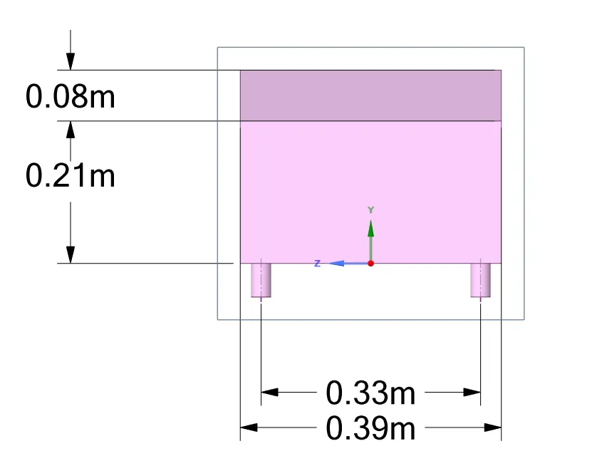
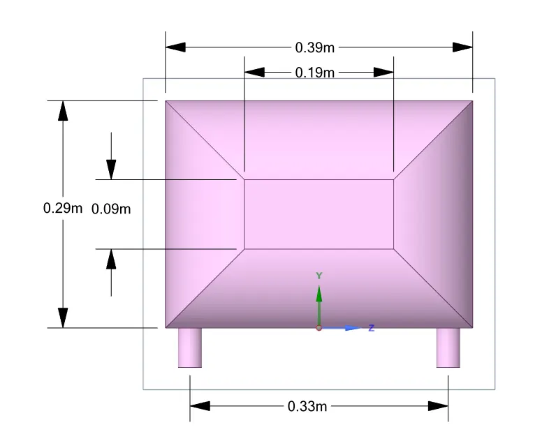
The geometry of the Ahmed body is shown below:
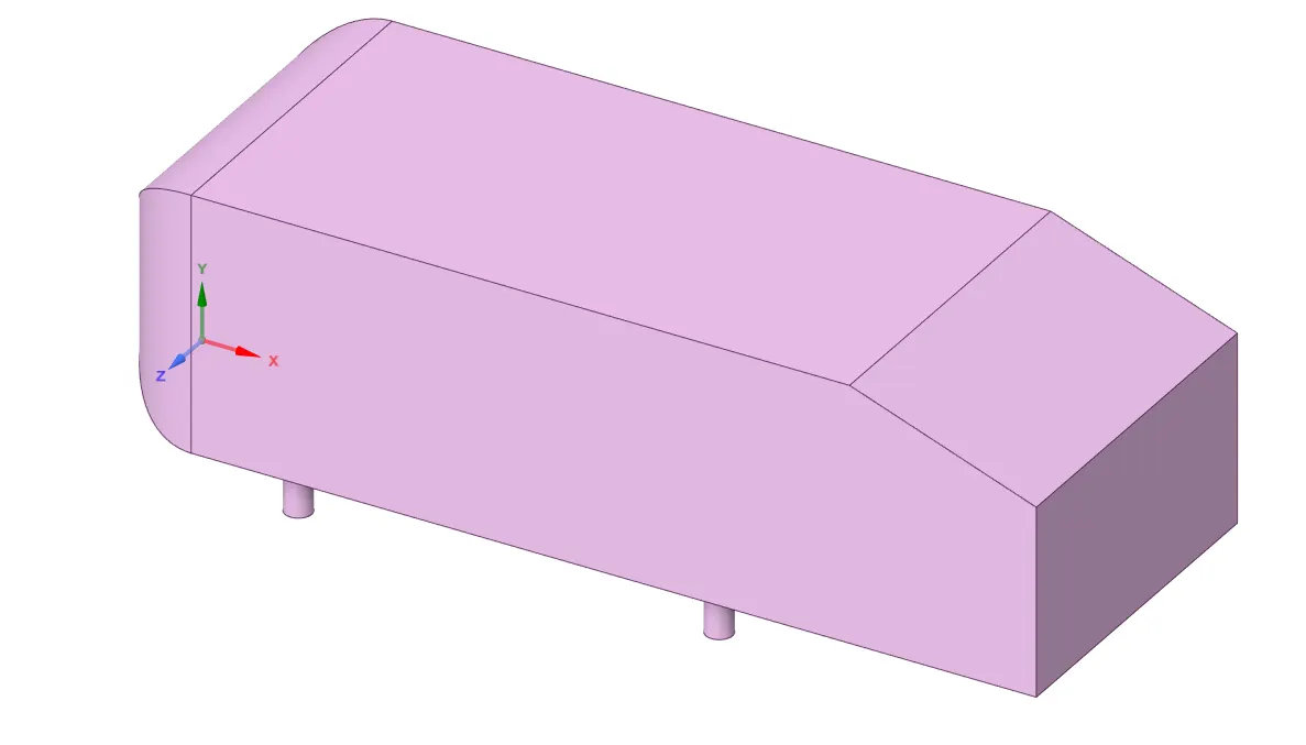
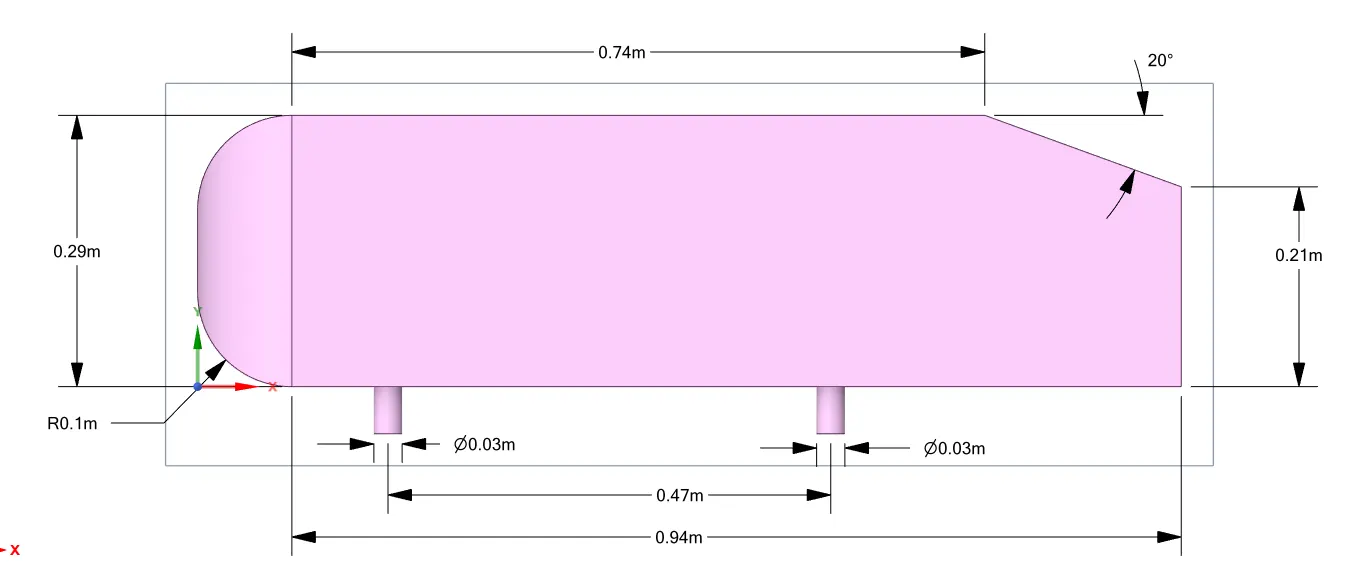
Ahmed body side view
Ahmed body rear view
Ahmed body front view
AREA=0.29*(0.39)=0.1131 `m^2`
Half of the area=0.05655 `m^2`
Length of Ahmed body=1.044 m
The inflation option utilizes the total thickness, determined based on the `y^+` value and the turbulence model employed. In this case, the k-omega turbulence model is used, requiring the `y^+` value to be within the range of 30 to 300.
Freestream velocity: `U_(infty)`=25m/s
Freestream density: `rho`=1.225 kg/`m^3`
Dynamic viscosity: `mu`=0.000017894 kg/(m s)
Length of Ahmed body: L=1.044 m
Desired `y^+`=100
Reynolds number:`Re = (rho * U_infty * L) / mu`=1786772.1023806867 >4000 (Turbulent model)
Skin friction coefficient:`C_f = 0.026 * Re^(-1/7)`=0.00332522173
Wall shear stress:`tau_(wall) = C_f * rho * (U_infty^2) / 2`=1.27293644352
Friction velocity:`U_f = sqrt(tau_(wall) / rho)`=1.01937813918
First layer thickness:`Delta_s = y^+ * mu / (U_f * rho)=1.432966**10^(-3)`m
Insert the calculated total thickness,and maximum of i=6 growth layers with growth ratio of r=1.2.
Total thickness = `Delta_i = Delta_s * r^(i - 1)`=3.566*10^(-3)` m
SOLVING & MODELING APPROACH -
The examination of external flow over the Ahmed body is conducted in a steady-state, given that the primary goal of the report is to illustrate the simulation and generate drag and lift plots. Initially, a basic mesh is employed for domain discretization to establish a baseline simulation. Subsequently, a systematic improvement of the mesh is undertaken through grid independence testing until results exhibit minimal variation. This analysis produces pressure and velocity contours, along with coefficient of drag and lift plots.
The k-epsilon, RSM, and LES models are predominantly suitable for turbulent core flows, which occur at a considerable distance from the wall. In contrast, the Spalart-Allamaras and K-Omega models are designed to be applicable throughout the boundary layer.
K-epsilon Model:
The K-epsilon model demonstrates elliptic near-wall behavior, which allows it to effectively interact with the wall and enforce Dirichlet boundary conditions. This behavior simplifies integration through the laminar sublayer without requiring additional numerically normalizing damping functions or two extra transport equations. However, in scenarios where flow integration through the viscous sublayer is required, such as in heat transfer, aerodynamic drag, or flow with an adverse pressure gradient, the k-omega model is preferred for simulating the flow over bodies like the Ahmed body.
K-Omega Model:
This model exhibits elliptic near-wall behavior, signifying its inherent capability to "communicate" with the wall and enforce Dirichlet boundary conditions. This behavior simplifies the integration through the laminar sublayer without the need for additional numerically normalizing damping functions or two extra transport equations. Instances where the flow necessitates integration through the viscous sublayer, such as in heat transfer, aerodynamic drag, or flow with an adverse pressure gradient, led to the utilization of the k-omega model for simulating the flow over the Ahmed body.
Configuring Geometry in SpaceClaim:
Given the perfect symmetry of the body, it is advantageous to simulate only half of it. This practice not only conserves computational resources by reducing the number of cells but also accelerates result generation. The provided geometry in the challenge requires a modification, a task well-suited for this stage of the course. Utilize the 'split body' command in SpaceClaim to execute the operation, and subsequently, apply the symmetry boundary condition in Fluent for conducting the simulation efficiently.
1. Load the model of the Ahmed body into SpaceClaim and convert the units from millimeters to meters.
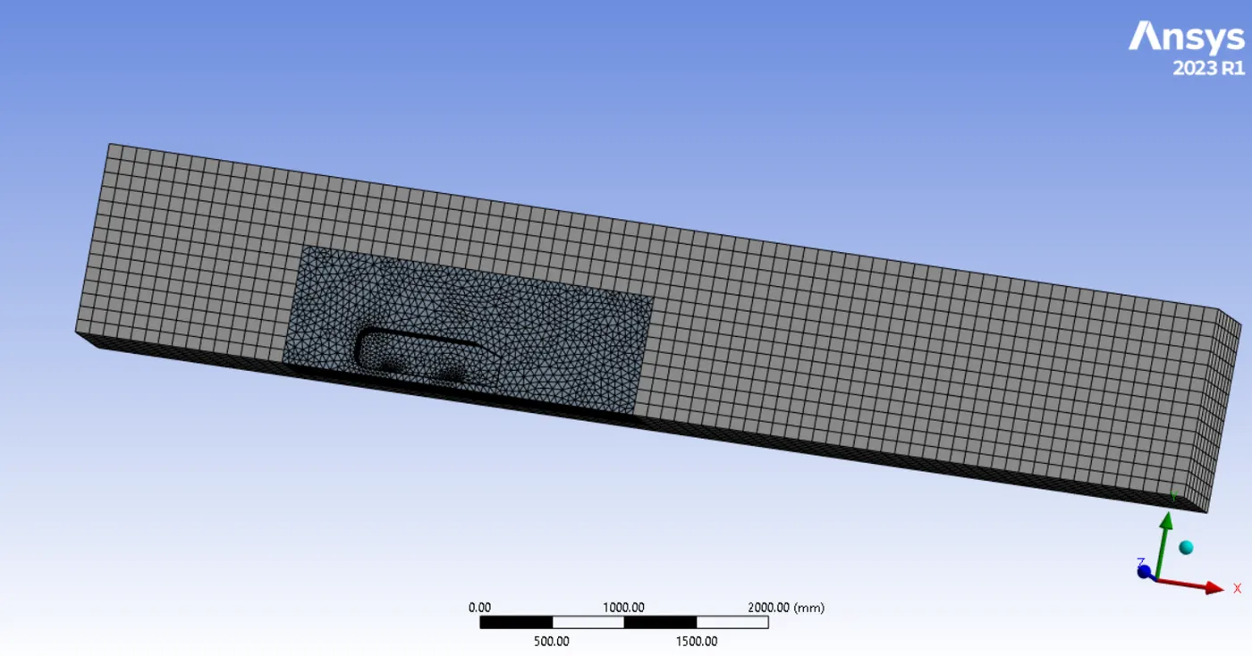
Navigate to the "Prepare" section, select the enclosure, and choose the Ahmed body. Input the enclosure dimensions as depicted in the snapshot below. Before providing the values, make sure to uncheck the symmetric option.
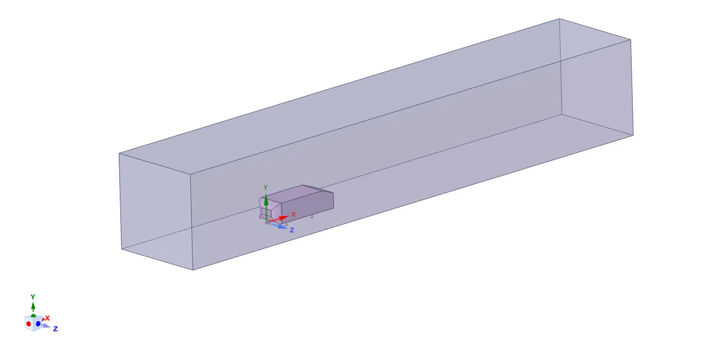
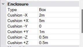
2. After completing the initial enclosure, we can establish an additional enclosure around the Ahmed body, allowing us to enhance mesh refinement within that space while effectively maintaining control over the overall cell count.
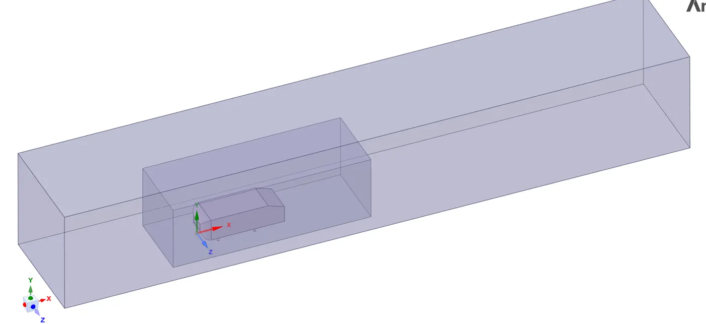
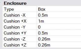
3. After creating both enclosures, we can examine interference and prevent mesh overlap in the second enclosure by utilizing the "Check Interference" function and removing any overlapping regions. This process is automated in SpaceClaim when the interference option is chosen within the "Prepare" section.
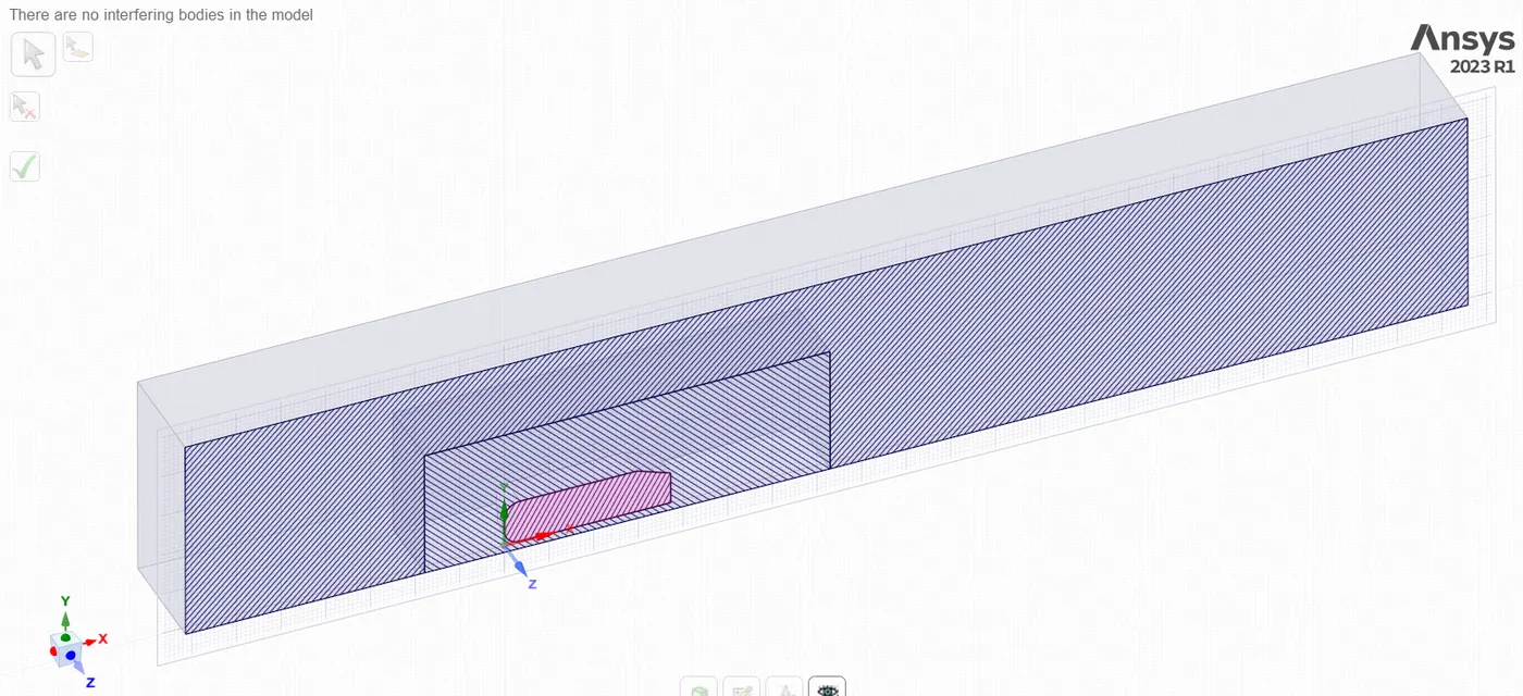
4. Following interference clearance, the next step involves splitting the body in half using the "Split Body" command in the design module. However, before proceeding, it's essential to create an XY plane at the origin to generate two equal halves. Select the "Design" option, choose "Planes," and position the cursor near the origin, then left-click. Three planes will appear; hide the unnecessary ones and utilize the XY plane. Now, choose "Split Body," select the relevant enclosure for splitting, pick the plane, and choose the part to be removed. Repeat the process to achieve the split for both enclosures and the body.
5. Mesh:
In this project, understanding the flow around the Ahmed body is crucial. To ensure accurate observation, refinement near the walls of the Ahmed body is necessary. This refinement is achieved through inflation. Inflation assists in generating body-fitted meshes that effectively capture the flow dynamics around the specific body.
To implement inflation:
- Right-click on the mesh
- Navigate to sizing
- In geometry, select the small enclosure
- For the boundary, choose the Ahmed body boundary layer.
Project Schematics:
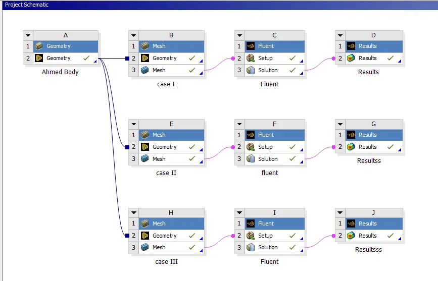
Case I:
Outer enclosure: 100mm(elemental size)
inner enclosure:50mm(elemental size)
Face sizing for Ahmed body :5mm(elemental size)
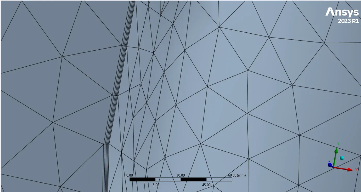
inflation for Ahmed body:6 layer with a total thickness of 3.566 mm
Generate mesh & will get inflation layers generated.
Mesh:
- Ensure the mesh is updated before opening Fluent.
- Perform mesh checking to ensure its quality and validity.
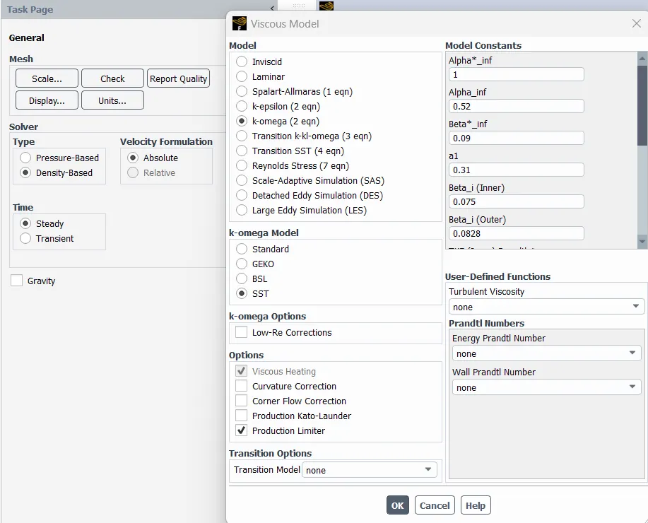
- Turbulence Model Selection:Choose the k−omega turbulence model, considering the relatively low inlet velocity of 25 m/s.
- Solver Configuration: Use the Density-based solver.
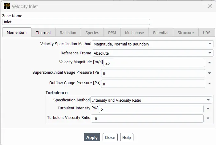
- Inlet Boundary Conditions: Set the inlet boundary condition with a velocity of 25 m/s.
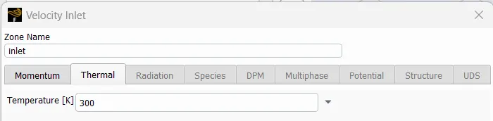
- Other boundary conditions:
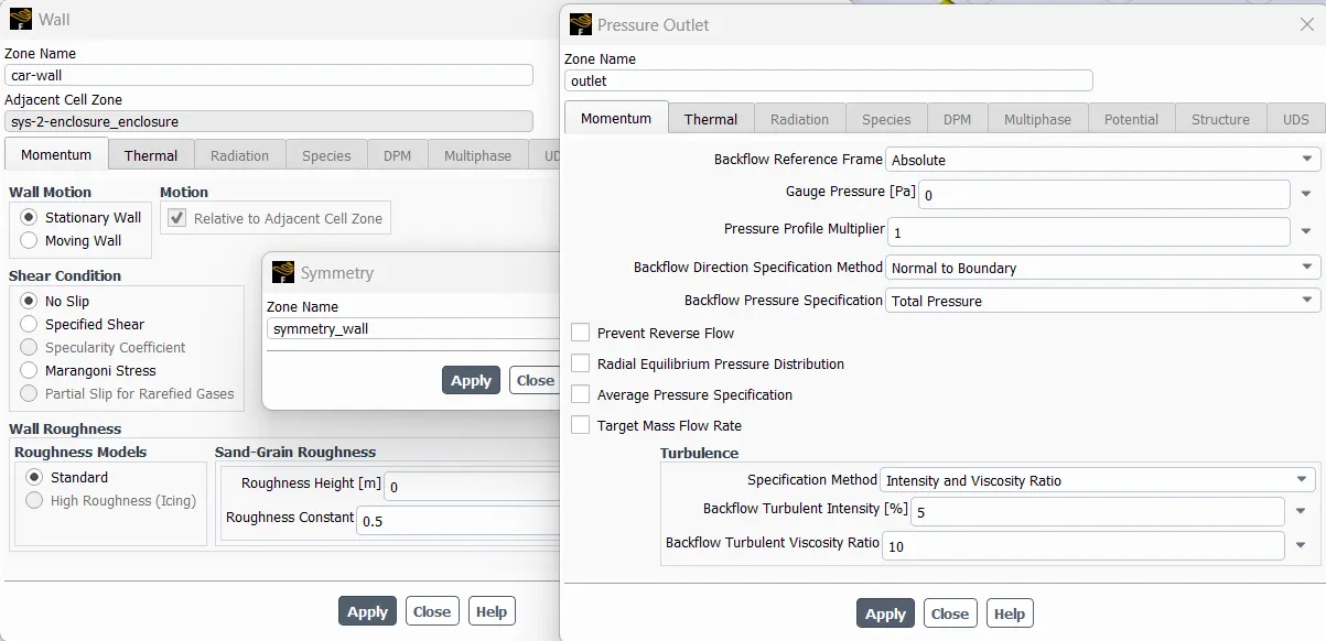
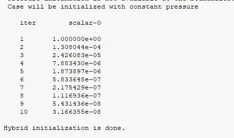
- Initialization: Initialize the solution to start the simulation.
- Post-Processing Steps: Proceed to the post-processing stage.
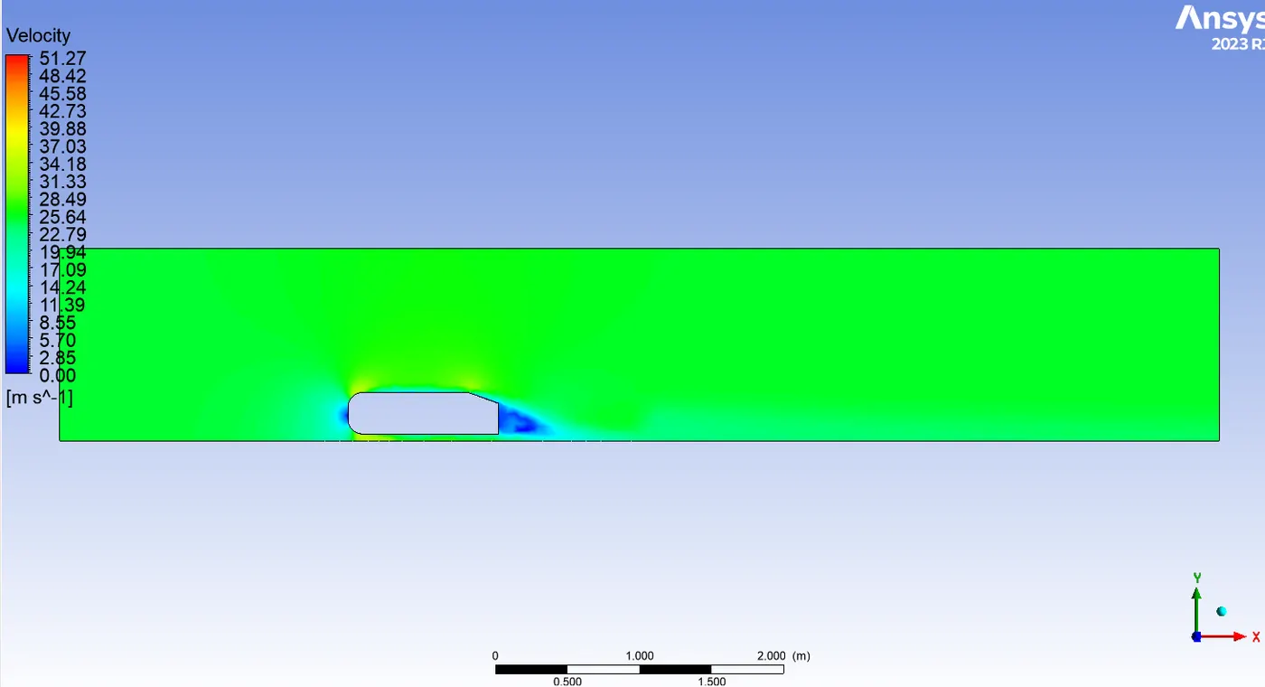
Velocity Profile: Create a cut plane to visualize the velocity profile.
Contour Plots: Generate contour plots for both pressure and velocity fields.
Drag and Lift Calculation: Utilize the definition tool to compute drag and lift. - Reference Values for Ahmed Body:
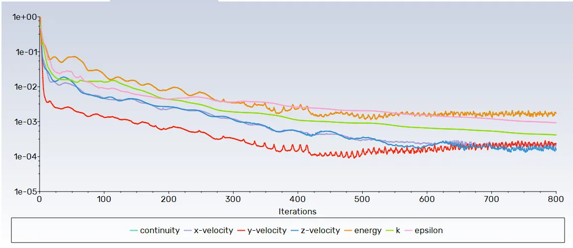
Provide the necessary reference values for the Ahmed body in the simulation. - Run Simulation: Run the simulation for some iterations to allow the solution to converge.
Residual Plots:
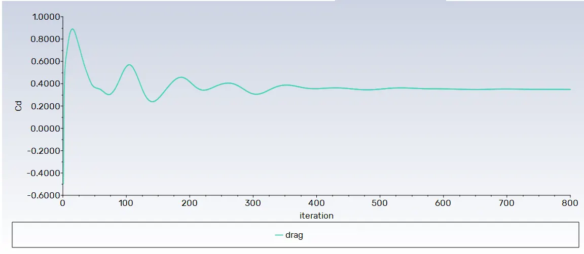
Coefficient of drag:
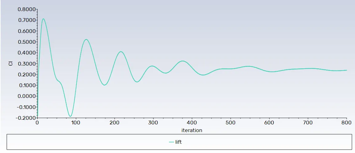
Coefficient of lift:
Velocity contour plot:
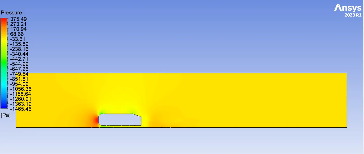
Pressure contour plot:
Velocity vector plot:
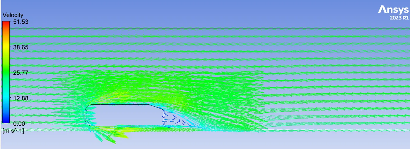
wake region:
Case II:
Outer enclosure: 80mm(elemental size)
inner enclosure:40mm(elemental size)
Face sizing for Ahmed body:5mm(elemental size)
inflation for Ahmed body:6 layer with a total thickness of 3.566 mm
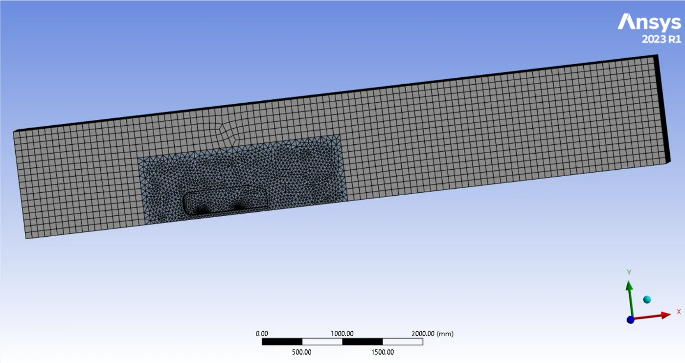
using same simulation configuration in fluent as case I, we get:
Residual Plots:
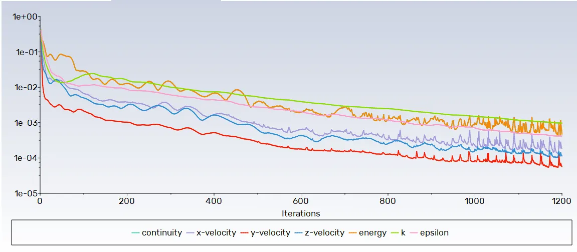
Coefficient of drag:
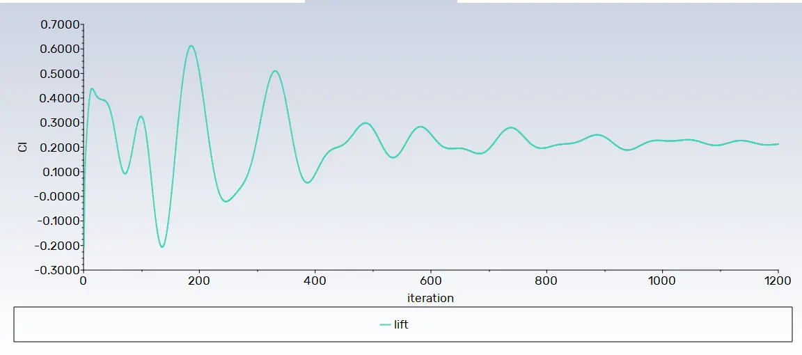
Coefficient of lift:
Velocity contour plot:
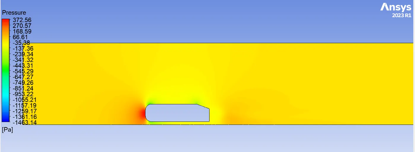
Pressure contour plot:
Velocity vector plot:
wake region:
Case III:
Outer enclosure: 60mm(elemental size)
inner enclosure:30mm(elemental size)
Face sizing for Ahmed body:5mm(elemental size)
inflation for Ahmed body:6 layer with a total thickness of 3.566 mm
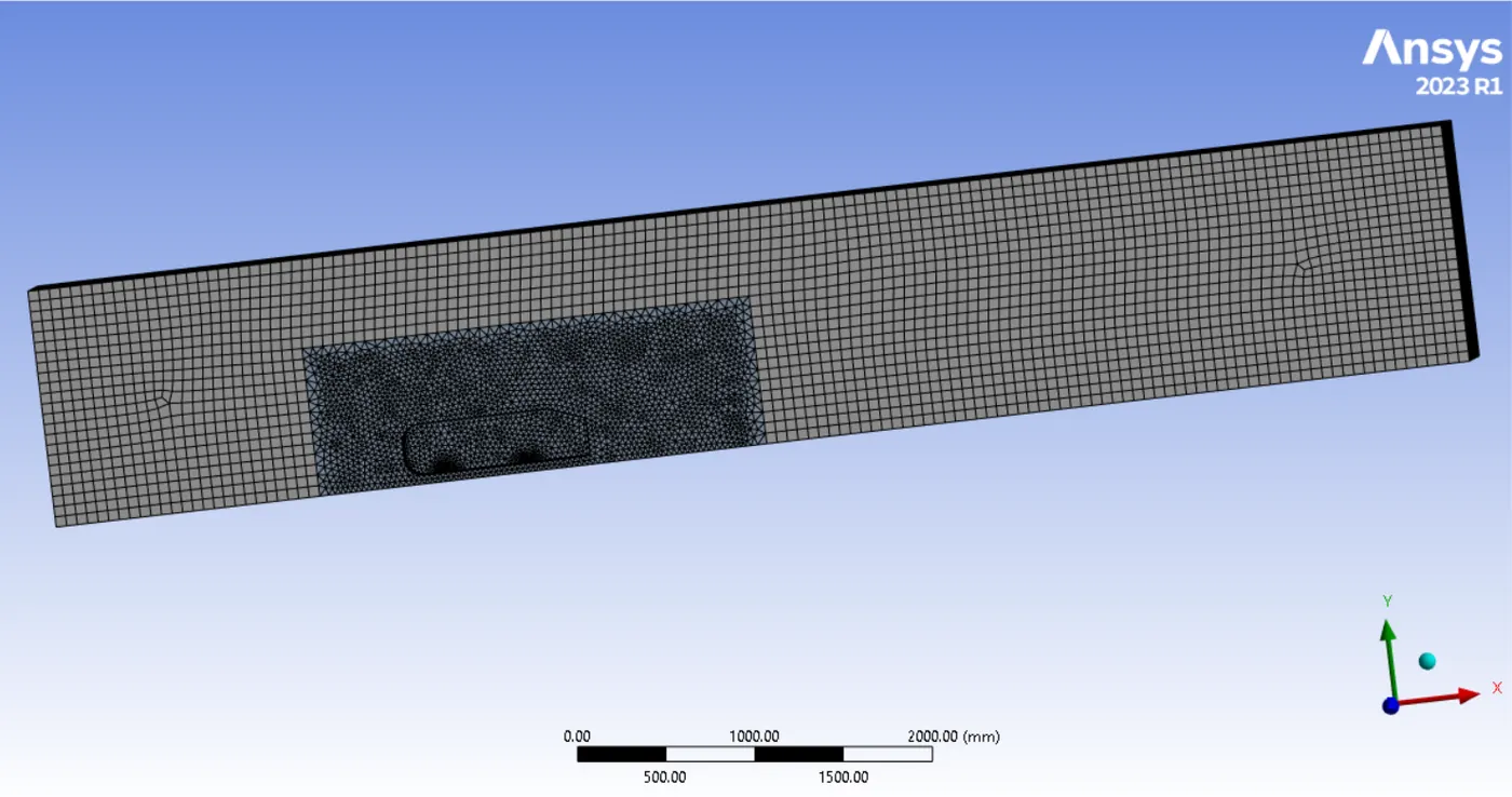
using same simulation configuration in fluent as case I, we get:
Residual Plots:
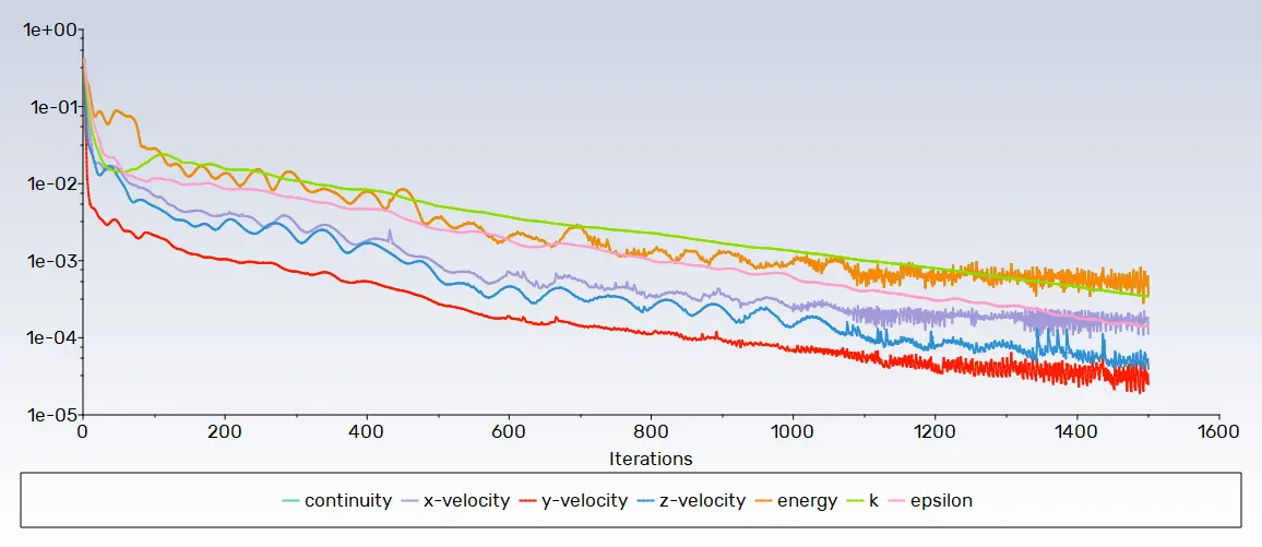
Coefficient of drag:
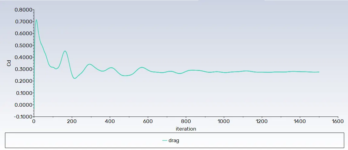
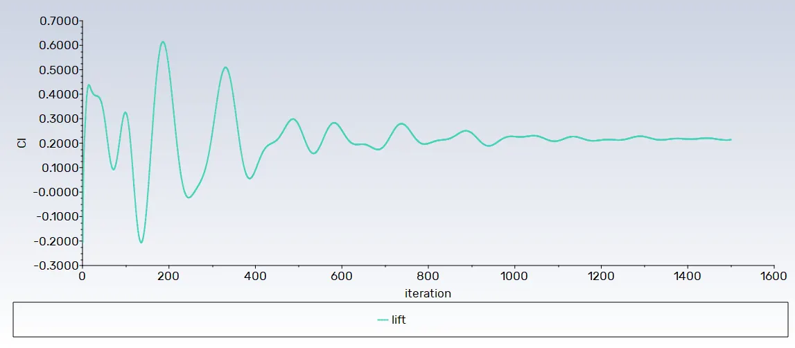
Coefficient of lift:
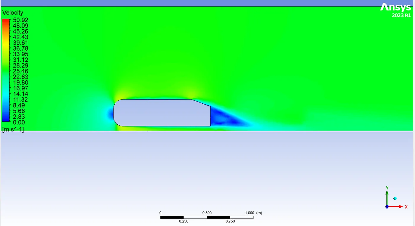
Velocity contour plot:
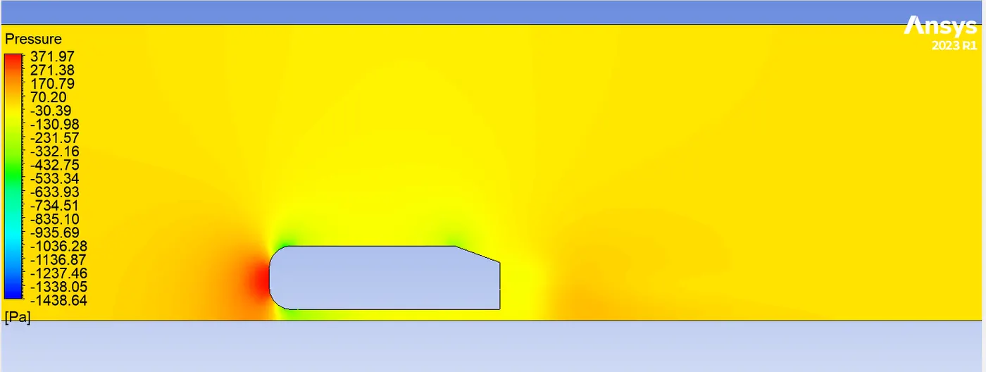
Pressure contour plot:
Velocity vector plot:
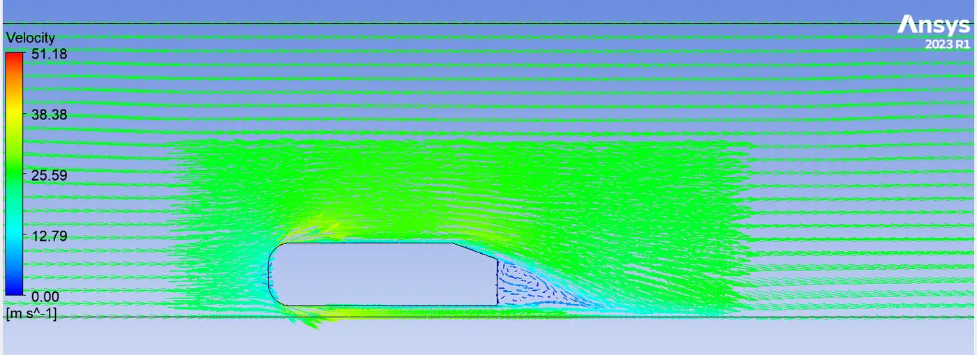
wake region:
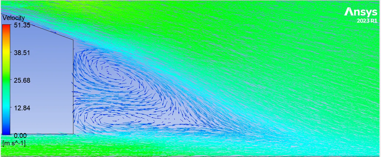
As the mesh is refined more the wake region is captured more properly.
------------------------------------------------------------------------------------------------------------------------------------------------------------------------------------------------------------------------------------------------------------------------------
Observations from the simulations:
- It is observed that refining the mesh in a computational simulation tends to result in an increase in computational time. This observation is based on the process of mesh refinement, which involves dividing the computational domain into smaller elements or cells to effectively capture more intricate features of the simulation, such as complex geometries or gradients. It is noted that, while a finer mesh can enhance result accuracy, it also entails a higher demand for computational resources.
- High Pressure zone is identified at the body's frontal section due to the accumulation of air flow at the front.
- Negative Pressure in Specific Regions: It's crucial to understand that negative pressure readings in certain areas do not indicate simulation errors. This is a characteristic of ANSYS and Fluent functionality.
- The term "pressure" displayed in ANSYS corresponds to gauge pressure. Gauge pressure is considered 0 when the total pressure aligns with atmospheric pressure.
- Negative "Pressure" Explanation: In instances where pressure readings appear negative, it is not an anomaly but rather an indication of pressure dropping below atmospheric conditions. Understanding this aspect is vital for accurate interpretation of simulation results.
Grid Independent Test:
Inflation for Ahmed body:6 layer with a total thickness of 3.566 mm
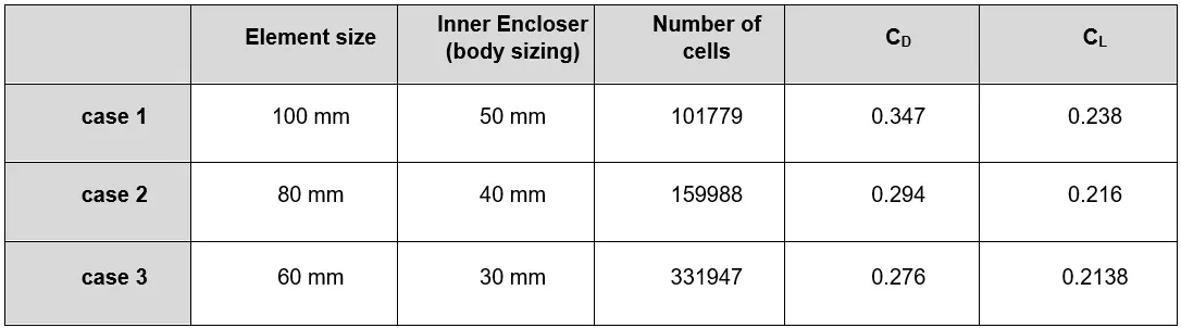
From the above table with the refinement of the mesh drag coefficient approaches closer to the analytical values that are because more cells are assigned at the boundary layer which results in more accurate results of drag coefficients.
Drag coeffcient decreases as number of elements increase, this claim is substantiated by the work of Jie Tian et al [3]
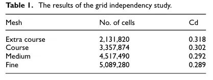
The key observation is that the drag coefficient remains relatively consistent when the mesh is refined, indicating grid independence. Conversely, the drag coefficient shows variability when the mesh is coarsened.
CONCLUSION:
- The grid independence test serves the purpose of identifying the optimal cell size required for convergence in simulations.
- Convergence is influenced by factors beyond mesh refinement, including Y+ value, inflation layer, and other setup parameters.
- With increasing refinement in the simulation setup, both drag and lift coefficients exhibit a decreasing trend.
- The Y+ value plays a critical role in determining drag, emphasizing the importance of achieving an appropriate Y+ value for accurate simulations.
- Negative pressure observed in the wake region is attributed to the absence of flow, influenced by factors such as separation and recirculation, as indicated by the vector plot near the wake region.
- Point of separation occurs at the rear end of the vehicle, extending beyond, where flow recirculates and reattaches to the boundary layer.
Study Gaps:
- The simulation uses default air properties, which may not represent real-world conditions accurately. Realistic scenarios may involve variations in temperature, pressure, or other properties. Need to extend the simulation to incorporate more realistic air properties, considering factors like temperature gradients, altitude effects, or changes in atmospheric conditions.
- The challenge does not address uncertainties associated with simulation results, such as variations in turbulence models, solver settings, or numerical discretization.To improve it is required perform an uncertainty analysis to assess the robustness of the simulation results under different modeling assumptions and parameters.
- Assuming perfect symmetry and simulating only half of Ahmed's body may not fully capture the intricacies of the flow patterns, especially in regions where asymmetry could play a role.
REFERENCES:
3.https://www.researchgate.net/publication/319041135_Aerodynamic_drag_reduction_and_flow_control_of_Ahmed_body_with_flaps/link/644e8fea5762c95ac3639027/download